使用 Optimum 和 Transformers Pipelines 進行加速推理

Optimum 現已支援推理，支援 Hugging Face Transformers pipelines，包括使用 ONNX Runtime 進行文字生成。

BERT 和 Transformers 的採用持續增長。基於 Transformer 的模型現在不僅在自然語言處理領域取得了最先進的效能，在計算機視覺、語音和時間序列領域也是如此。💬 🖼 🎤 ⏳

公司現在正從實驗和研究階段轉向生產階段，以便將 Transformer 模型用於大規模工作負載。但預設情況下，BERT 及其同類模型與傳統的機器學習演算法相比，相對較慢、較大且複雜。

為了解決這個挑戰，我們建立了 Optimum——它是 Hugging Face Transformers 的一個擴充套件，旨在加速像 BERT 這樣的 Transformer 模型的訓練和推理。

在這篇博文中，你將學到

• 1. 什麼是 Optimum？ELI5 (給 5 歲小孩的解釋)
• 2. 新的 Optimum 推理和 pipeline 特性
• 3. 加速 RoBERTa 用於問答任務的端到端教程，包括量化和最佳化
• 4. 當前的侷限性
• 5. Optimum 推理常見問題解答
• 6. 接下來是什麼？

讓我們開始吧！🚀

1. 什麼是 Optimum？ELI5 (給 5 歲小孩的解釋)

Hugging Face Optimum 是一個開源庫，是 Hugging Face Transformers 的擴充套件，它提供了一套統一的效能最佳化工具 API，以在加速硬體上訓練和執行模型時實現最高效率，包括用於在 Graphcore IPU 和 Habana Gaudi 上最佳化效能的工具包。Optimum 可用於加速訓練、量化、圖最佳化，現在也支援 transformers pipelines 的推理。

2. 新的 Optimum 推理和 pipeline 特性

隨著 Optimum 1.2 的釋出，我們增加了對推理和 transformers pipelines 的支援。這使得 Optimum 使用者可以利用他們習慣的 transformers API，並結合像 ONNX Runtime 這樣的加速執行時的強大功能。

從 Transformers 切換到 Optimum 推理 Optimum 推理模型在 API 上與 Hugging Face Transformers 模型相容。這意味著你只需將你的 AutoModelForXxx 類替換為 Optimum 中相應的 ORTModelForXxx 類。例如，以下是如何在 Optimum 中使用問答模型：

from transformers import AutoTokenizer, pipeline
-from transformers import AutoModelForQuestionAnswering
+from optimum.onnxruntime import ORTModelForQuestionAnswering

-model = AutoModelForQuestionAnswering.from_pretrained("deepset/roberta-base-squad2") # pytorch checkpoint
+model = ORTModelForQuestionAnswering.from_pretrained("optimum/roberta-base-squad2") # onnx checkpoint
tokenizer = AutoTokenizer.from_pretrained("deepset/roberta-base-squad2")

optimum_qa = pipeline("question-answering", model=model, tokenizer=tokenizer)

question = "What's my name?"
context = "My name is Philipp and I live in Nuremberg."
pred = optimum_qa(question, context)

在第一個版本中，我們添加了對 ONNX Runtime 的支援，未來還會有更多！這些新的 ORTModelForXX 現在可以與 transformers pipelines 一起使用。它們也完全整合到 Hugging Face Hub 中，可以從社群推送和拉取最佳化的檢查點。此外，你可以使用 ORTQuantizer 和 ORTOptimizer 先對模型進行量化和最佳化，然後再進行推理。檢視加速 RoBERTa 用於問答任務的端到端教程，包括量化和最佳化瞭解更多詳情。

3. 加速 RoBERTa 用於問答任務的端到端教程，包括量化和最佳化

在這個加速 RoBERTa 用於問答任務的端到端教程中，你將學到如何：

1. 為 ONNX Runtime 安裝 Optimum
2. 將 Hugging Face Transformers 模型轉換為 ONNX 以進行推理
3. 使用 ORTOptimizer 最佳化模型
4. 使用 ORTQuantizer 應用動態量化
5. 使用 Transformers pipelines 執行加速推理
6. 評估效能和速度

讓我們開始吧 🚀

本教程是在一個 m5.xlarge AWS EC2 例項上建立和執行的。

3.1 為 Onnxruntime 安裝 Optimum

我們的第一步是安裝帶有 onnxruntime 實用工具的 Optimum。

pip install "optimum[onnxruntime]==1.2.0"

這將為我們安裝所有必需的包，包括 transformers、torch 和 onnxruntime。如果你要使用 GPU，可以用 pip install optimum[onnxruntime-gpu] 來安裝 optimum。

3.2 將 Hugging Face Transformers 模型轉換為 ONNX 以進行推理**

在我們開始最佳化之前，我們需要將我們的普通 transformers 模型轉換為 onnx 格式。為此，我們將使用新的 ORTModelForQuestionAnswering 類，並呼叫帶 from_transformers 屬性的 from_pretrained() 方法。我們使用的模型是 deepset/roberta-base-squad2，一個在 SQUAD2 資料集上微調的 RoBERTa 模型，F1 分數達到 82.91，其任務 (feature) 為 question-answering。

from pathlib import Path
from transformers import AutoTokenizer, pipeline
from optimum.onnxruntime import ORTModelForQuestionAnswering

model_id = "deepset/roberta-base-squad2"
onnx_path = Path("onnx")
task = "question-answering"

# load vanilla transformers and convert to onnx
model = ORTModelForQuestionAnswering.from_pretrained(model_id, from_transformers=True)
tokenizer = AutoTokenizer.from_pretrained(model_id)

# save onnx checkpoint and tokenizer
model.save_pretrained(onnx_path)
tokenizer.save_pretrained(onnx_path)

# test the model with using transformers pipeline, with handle_impossible_answer for squad_v2
optimum_qa = pipeline(task, model=model, tokenizer=tokenizer, handle_impossible_answer=True)
prediction = optimum_qa(question="What's my name?", context="My name is Philipp and I live in Nuremberg.")

print(prediction)
# {'score': 0.9041663408279419, 'start': 11, 'end': 18, 'answer': 'Philipp'}

我們成功地將我們的普通 transformers 模型轉換成了 onnx 格式，並使用 transformers.pipelines 運行了第一次預測。現在，讓我們來最佳化它。🏎

如果你想了解更多關於匯出 transformers 模型的資訊，請檢視文件：匯出 🤗 Transformers 模型

3.3 使用 ORTOptimizer 最佳化模型

將 onnx 檢查點儲存到 onnx/ 後，我們現在可以使用 ORTOptimizer 來應用圖最佳化，例如運算元融合和常量摺疊，以加速延遲和推理。

from optimum.onnxruntime import ORTOptimizer
from optimum.onnxruntime.configuration import OptimizationConfig

# create ORTOptimizer and define optimization configuration
optimizer = ORTOptimizer.from_pretrained(model_id, feature=task)
optimization_config = OptimizationConfig(optimization_level=99) # enable all optimizations

# apply the optimization configuration to the model
optimizer.export(
    onnx_model_path=onnx_path / "model.onnx",
    onnx_optimized_model_output_path=onnx_path / "model-optimized.onnx",
    optimization_config=optimization_config,
)

為了測試效能，我們可以再次使用 ORTModelForQuestionAnswering 類，並提供一個額外的 file_name 引數來載入我們最佳化後的模型。（這也適用於 Hub 上可用的模型）。

from optimum.onnxruntime import ORTModelForQuestionAnswering

# load quantized model
opt_model = ORTModelForQuestionAnswering.from_pretrained(onnx_path, file_name="model-optimized.onnx")

# test the quantized model with using transformers pipeline
opt_optimum_qa = pipeline(task, model=opt_model, tokenizer=tokenizer, handle_impossible_answer=True)
prediction = opt_optimum_qa(question="What's my name?", context="My name is Philipp and I live in Nuremberg.")
print(prediction)
# {'score': 0.9041663408279419, 'start': 11, 'end': 18, 'answer': 'Philipp'}

我們將在步驟 3.6 評估效能和速度 中詳細評估效能變化。

3.4 使用 ORTQuantizer 應用動態量化

最佳化模型後，我們可以使用 ORTQuantizer 對其進行量化以進一步加速。ORTOptimizer 可用於應用動態量化，以減小模型大小並加速延遲和推理。

我們使用 avx512_vnni，因為例項由支援 avx512 的英特爾 Cascade Lake CPU 驅動。

from optimum.onnxruntime import ORTQuantizer
from optimum.onnxruntime.configuration import AutoQuantizationConfig

# create ORTQuantizer and define quantization configuration
quantizer = ORTQuantizer.from_pretrained(model_id, feature=task)
qconfig = AutoQuantizationConfig.avx512_vnni(is_static=False, per_channel=True)

# apply the quantization configuration to the model
quantizer.export(
    onnx_model_path=onnx_path / "model-optimized.onnx",
    onnx_quantized_model_output_path=onnx_path / "model-quantized.onnx",
    quantization_config=qconfig,
)

我們現在可以比較這個模型的尺寸以及一些延遲效能

import os
# get model file size
size = os.path.getsize(onnx_path / "model.onnx")/(1024*1024)
print(f"Vanilla Onnx Model file size: {size:.2f} MB")
size = os.path.getsize(onnx_path / "model-quantized.onnx")/(1024*1024)
print(f"Quantized Onnx Model file size: {size:.2f} MB")

# Vanilla Onnx Model file size: 473.31 MB
# Quantized Onnx Model file size: 291.77 MB

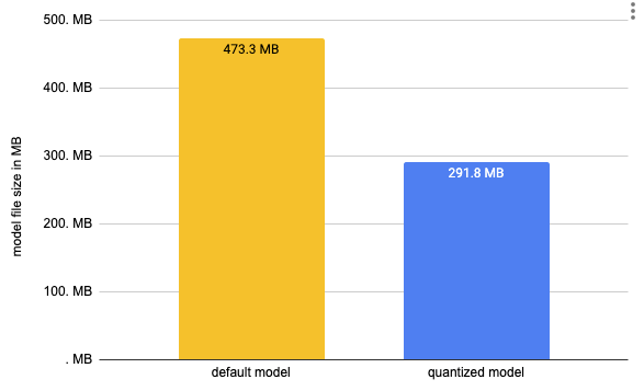
我們已將模型大小從 473MB 減小到 291MB，減小了近 50%。要執行推理，我們可以再次使用 ORTModelForQuestionAnswering 類，並提供一個額外的 file_name 引數來載入我們量化後的模型。（這也適用於 Hub 上可用的模型）。

# load quantized model
quantized_model = ORTModelForQuestionAnswering.from_pretrained(onnx_path, file_name="model-quantized.onnx")

# test the quantized model with using transformers pipeline
quantized_optimum_qa = pipeline(task, model=quantized_model, tokenizer=tokenizer, handle_impossible_answer=True)
prediction = quantized_optimum_qa(question="What's my name?", context="My name is Philipp and I live in Nuremberg.")
print(prediction)
# {'score': 0.9246969819068909, 'start': 11, 'end': 18, 'answer': 'Philipp'}

不錯！模型預測了相同的答案。

3.5 使用 Transformers pipelines 執行加速推理

Optimum 內建支援 transformers pipelines。這使我們能夠利用我們熟悉的 PyTorch 和 TensorFlow 模型 API。我們已經在步驟 3.2、3.3 和 3.4 中使用了此功能來測試我們轉換和最佳化後的模型。在撰寫本文時，我們支援 ONNX Runtime，未來還會支援更多。下面是一個如何使用 transformers pipelines 的示例。

from transformers import AutoTokenizer, pipeline
from optimum.onnxruntime import ORTModelForQuestionAnswering

tokenizer = AutoTokenizer.from_pretrained(onnx_path)
model = ORTModelForQuestionAnswering.from_pretrained(onnx_path)

optimum_qa = pipeline("question-answering", model=model, tokenizer=tokenizer)
prediction = optimum_qa(question="What's my name?", context="My name is Philipp and I live in Nuremberg.")

print(prediction)
# {'score': 0.9041663408279419, 'start': 11, 'end': 18, 'answer': 'Philipp'}

此外，我們還為 Optimum 添加了一個 pipelines API，以為您的加速模型提供更多安全性。這意味著如果您嘗試將 optimum.pipelines 與不支援的模型或任務一起使用，您會看到一個錯誤。您可以將 optimum.pipelines 作為 transformers.pipelines 的替代品。

from transformers import AutoTokenizer
from optimum.onnxruntime import ORTModelForQuestionAnswering
from optimum.pipelines import pipeline

tokenizer = AutoTokenizer.from_pretrained(onnx_path)
model = ORTModelForQuestionAnswering.from_pretrained(onnx_path)

optimum_qa = pipeline("question-answering", model=model, tokenizer=tokenizer, handle_impossible_answer=True)
prediction = optimum_qa(question="What's my name?", context="My name is Philipp and I live in Nuremberg.")

print(prediction)
# {'score': 0.9041663408279419, 'start': 11, 'end': 18, 'answer': 'Philipp'}

3.6 評估效能和速度

在這個加速 RoBERTa 用於問答任務的端到端教程（包括量化和最佳化）中，我們建立了 3 個不同的模型。一個普通轉換的模型，一個最佳化過的模型，以及一個量化過的模型。

作為本教程的最後一步，我們想詳細看看我們模型的效能和準確性。應用最佳化技術，如圖最佳化或量化，不僅會影響效能（延遲），也可能對模型的準確性產生影響。所以加速你的模型是有權衡的。

讓我們來評估我們的模型。我們的 transformers 模型 deepset/roberta-base-squad2 是在 SQUAD2 資料集上微調的。這將是我們用來評估我們模型的資料集。

from datasets import load_metric,load_dataset

metric = load_metric("squad_v2")
dataset = load_dataset("squad_v2")["validation"]

print(f"length of dataset {len(dataset)}")
#length of dataset 11873

我們現在可以利用 datasets 的 map 函式來遍歷 squad 2 的驗證集，併為每個資料點執行預測。因此，我們編寫一個 evaluate 輔助方法，它使用我們的 pipelines 並應用一些轉換來處理 squad v2 指標。

這可能需要相當長的時間（1.5 小時）

def evaluate(example):
  default = optimum_qa(question=example["question"], context=example["context"])
  optimized = opt_optimum_qa(question=example["question"], context=example["context"])
  quantized = quantized_optimum_qa(question=example["question"], context=example["context"])
  return {
      'reference': {'id': example['id'], 'answers': example['answers']},
      'default': {'id': example['id'],'prediction_text': default['answer'], 'no_answer_probability': 0.},
      'optimized': {'id': example['id'],'prediction_text': optimized['answer'], 'no_answer_probability': 0.},
      'quantized': {'id': example['id'],'prediction_text': quantized['answer'], 'no_answer_probability': 0.},
      }

result = dataset.map(evaluate)
# COMMENT IN to run evaluation on 2000 subset of the dataset
# result = dataset.shuffle().select(range(2000)).map(evaluate)

現在讓我們來比較結果

default_acc = metric.compute(predictions=result["default"], references=result["reference"])
optimized = metric.compute(predictions=result["optimized"], references=result["reference"])
quantized = metric.compute(predictions=result["quantized"], references=result["reference"])

print(f"vanilla model: exact={default_acc['exact']}% f1={default_acc['f1']}%")
print(f"optimized model: exact={optimized['exact']}% f1={optimized['f1']}%")
print(f"quantized model: exact={quantized['exact']}% f1={quantized['f1']}%")

# vanilla model: exact=79.07858165585783% f1=82.14970024570314%
# optimized model: exact=79.07858165585783% f1=82.14970024570314%
# quantized model: exact=78.75010528088941% f1=81.82526107204629%

我們最佳化和量化後的模型實現了 78.75% 的精確匹配和 81.83% 的 f1 分數，這是原始準確率的 99.61%。達到原始模型的 99% 已經非常好了，特別是考慮到我們使用了動態量化。

好的，讓我們測試一下我們最佳化和量化後模型的效能（延遲）。

但首先，讓我們將上下文和問題擴充套件到一個更有意義的序列長度，即 128。

context="Hello, my name is Philipp and I live in Nuremberg, Germany. Currently I am working as a Technical Lead at Hugging Face to democratize artificial intelligence through open source and open science. In the past I designed and implemented cloud-native machine learning architectures for fin-tech and insurance companies. I found my passion for cloud concepts and machine learning 5 years ago. Since then I never stopped learning. Currently, I am focusing myself in the area NLP and how to leverage models like BERT, Roberta, T5, ViT, and GPT2 to generate business value."
question="As what is Philipp working?"

為了簡單起見，我們將使用一個 Python 迴圈來計算我們的原始模型以及最佳化和量化後模型的平均/均值延遲。

from time import perf_counter
import numpy as np

def measure_latency(pipe):
    latencies = []
    # warm up
    for _ in range(10):
        _ = pipe(question=question, context=context)
    # Timed run
    for _ in range(100):
        start_time = perf_counter()
        _ =  pipe(question=question, context=context)
        latency = perf_counter() - start_time
        latencies.append(latency)
    # Compute run statistics
    time_avg_ms = 1000 * np.mean(latencies)
    time_std_ms = 1000 * np.std(latencies)
    return f"Average latency (ms) - {time_avg_ms:.2f} +\- {time_std_ms:.2f}"

print(f"Vanilla model {measure_latency(optimum_qa)}")
print(f"Optimized & Quantized model {measure_latency(quantized_optimum_qa)}")

# Vanilla model Average latency (ms) - 117.61 +\- 8.48
# Optimized & Quantized model Average latency (ms) - 64.94 +\- 3.65

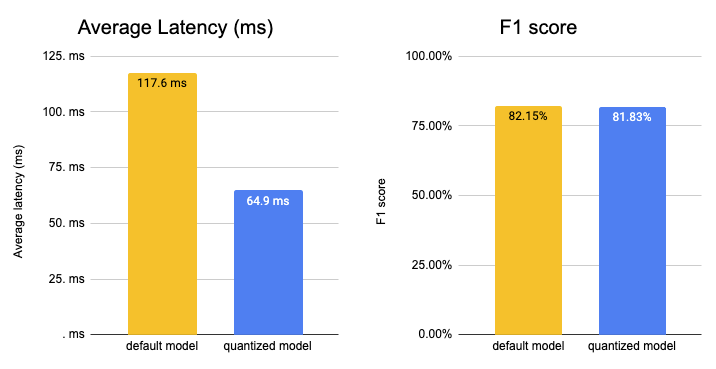
我們成功地將模型的延遲從 117.61ms 加速到 64.94ms，大約快了 2 倍，同時保持了 99.61% 的準確率。我們應該記住的是，我們使用的是一箇中等效能的 CPU 例項，擁有 2 個物理核心。透過切換到 GPU 或更高效能的 CPU 例項，例如由 ice-lake 驅動的例項，您可以將延遲數字降低到幾毫秒。

4. 當前的侷限性

我們剛剛開始在 https://github.com/huggingface/optimum 中支援推理，所以我們也想分享一下當前的侷限性。所有這些侷限性都在我們的路線圖上，並將在不久的將來得到解決。

• 大於 2GB 的遠端模型： 目前，只能從 Hugging Face Hub 載入小於 2GB 的模型。我們正在努力增加對大於 2GB 的模型/多檔案模型的支援。
• Seq2Seq 任務/模型： 我們尚不支援 seq2seq 任務，例如摘要和像 T5 這樣的模型，這主要是由於對單個模型的支援有限。但我們正在積極努力解決這個問題，以便為您提供與在 transformers 中熟悉的相同體驗。
• Past key values (過去鍵值)： 像 GPT-2 這樣的生成模型使用一種叫做過去鍵值的東西，它們是注意力塊的預計算鍵值對，可以用來加速解碼。目前 ORTModelForCausalLM 尚未使用過去鍵值。
• 無快取： 目前載入最佳化後的模型 (*.onnx) 時，它不會被本地快取。

5. Optimum 推理常見問題解答

支援哪些任務？

你可以在文件中找到所有支援任務的列表。目前支援的 pipelines 任務有 `feature-extraction`、`text-classification`、`token-classification`、`question-answering`、`zero-shot-classification`、`text-generation`。

支援哪些模型？

任何可以使用 transformers.onnx 匯出並且有支援任務的模型都可以使用，這包括 BERT、ALBERT、GPT2、RoBERTa、XLM-RoBERTa、DistilBERT 等。

支援哪些執行時？

目前支援 ONNX Runtime。我們正在努力在未來新增更多。如果您對特定的執行時感興趣，請告訴我們。

如何將 Optimum 與 Transformers 一起使用？

您可以在我們的文件中找到示例和說明。

如何使用 GPU？

要使用 GPU，您只需安裝 optimum[onnxruntine-gpu]，它將安裝所需的 GPU 提供程式並預設使用它們。

如何將量化和最佳化後的模型與 pipelines 一起使用？

您可以使用新的 ORTModelForXXX 類，透過 from_pretrained 方法載入最佳化或量化後的模型。您可以在我們的文件中瞭解更多資訊。

6. 接下來是什麼？

你問 Optimum 的下一步是什麼？有很多事情。我們專注於使 Optimum 成為用於加速和最佳化 transformers 的參考開源工具包。為了實現這一點，我們將解決當前的限制，改進文件，建立更多內容和示例，並推動加速和最佳化 transformers 的極限。

除了當前的限制之外，Optimum 路線圖上的一些重要功能包括：

• 支援語音模型 (Wav2vec2) 和語音任務 (自動語音識別)
• 支援視覺模型 (ViT) 和視覺任務 (影像分類)
• 透過增加對 OrtValue 和 IOBinding 的支援來提高效能
• 更簡便地評估加速模型的方法
• 增加對其他執行時和提供商的支援，如 TensorRT 和 AWS-Neuron

---

感謝閱讀！如果您和我一樣對加速 Transformers、提高其效率並將其擴充套件到數十億次請求感到興奮，那麼您應該申請，我們正在招聘。🚀

如果您有任何問題，請隨時透過 Github 或論壇與我聯絡。您也可以在 Twitter 或 LinkedIn 上與我聯絡。