利用預訓練語言模型檢查點進行編碼器-解碼器模型訓練


Vaswani 等人(2017)提出了基於 Transformer 的編碼器-解碼器模型,最近受到了廣泛關注,例如 Lewis 等人(2019)、Raffel 等人(2019)、Zhang 等人(2020)、Zaheer 等人(2020)、Yan 等人(2020)。
與 BERT 和 GPT2 類似,大型預訓練編碼器-解碼器模型已顯示出在各種序列到序列任務中顯著提升效能,例如 Lewis 等人(2019)、Raffel 等人(2019)。然而,由於預訓練編碼器-解碼器模型的計算成本巨大,此類模型的開發主要侷限於大型公司和機構。
在《Leveraging Pre-trained Checkpoints for Sequence Generation Tasks》(2020)中,Sascha Rothe、Shashi Narayan 和 Aliaksei Severyn 利用預訓練的僅編碼器和/或僅解碼器檢查點(例如 BERT、GPT2)來初始化編碼器-解碼器模型,以跳過昂貴的預訓練過程。作者表明,此類溫啟動編碼器-解碼器模型在多種序列到序列任務上,僅需一小部分訓練成本即可獲得與大型預訓練編碼器-解碼器模型(如T5和Pegasus)相媲美的結果。
在本筆記本中,我們將詳細解釋如何溫啟動編碼器-解碼器模型,根據Rothe 等人(2020)的論文提供實用技巧,最後透過一個完整的程式碼示例,展示如何使用 🤗Transformers 溫啟動編碼器-解碼器模型。
本筆記本分為 4 個部分
- 引言 - 對 NLP 中預訓練語言模型以及溫啟動編碼器-解碼器模型的需求進行簡要總結。
- 編碼器-解碼器模型的溫啟動(理論) - 圖解說明編碼器-解碼器模型是如何進行溫啟動的?
- 編碼器-解碼器模型的溫啟動(分析) - 《Leveraging Pre-trained Checkpoints for Sequence Generation Tasks》(2020)摘要 - 哪些模型組合對溫啟動編碼器-解碼器模型有效;它在不同任務之間有何差異?
- 使用 🤗Transformers 溫啟動編碼器-解碼器模型(實踐) - 詳細展示如何使用
EncoderDecoderModel框架溫啟動基於 Transformer 的編碼器-解碼器模型的完整程式碼示例。
強烈建議(甚至可能是必要)閱讀這篇博文,瞭解基於 Transformer 的編碼器-解碼器模型。
我們首先介紹溫啟動編碼器-解碼器模型的背景。
引言
最近,預訓練語言模型徹底改變了自然語言處理(NLP)領域。
最早的預訓練語言模型是基於迴圈神經網路(RNN),由Dai 等人(2015)提出。Dai 等人表明,在未標註資料上預訓練基於 RNN 的模型,然後針對特定任務進行微調,比直接在任務上訓練隨機初始化的模型效果更好。然而,直到 2018 年,預訓練語言模型才在 NLP 領域被廣泛接受。Peters 等人提出的 ELMO和Howard 等人提出的 ULMFit是首批顯著提升一系列自然語言理解(NLU)任務最新技術的預訓練語言模型。僅僅幾個月後,OpenAI 和 Google 釋出了基於 Transformer 的預訓練語言模型,分別命名為Radford 等人提出的 GPT和Devlin 等人提出的 BERT。基於 Transformer 的語言模型在效率上優於 RNN,使得 GPT2 和 BERT 能夠在大量未標註文字資料上進行預訓練。一旦預訓練完成,BERT 和 GPT 被證明只需要很少的微調即可在十多個 NLU 任務上打破最新技術水平。
預訓練語言模型將任務無關知識有效地遷移到任務特定知識的能力,極大地推動了 NLU 的發展。工程師和研究人員以前需要從頭開始訓練語言模型,而現在,公開可用的、大型預訓練語言模型的檢查點可以在極短的時間內以極低的成本進行微調。這在工業界可以節省數百萬美元,在研究中則可以實現更快的原型開發和更好的基準測試。
預訓練語言模型已經在 NLU 任務上確立了新的效能水平,越來越多的研究都建立在利用這些預訓練語言模型來改進 NLU 系統上。然而,獨立的 BERT 和 GPT 模型在序列到序列任務上(例如,文字摘要、機器翻譯、句子改寫等)的表現則不盡如人意。
序列到序列任務定義為將輸入序列 對映到輸出序列 ,其中輸出長度 是預先未知的。因此,序列到序列模型應該定義輸出序列 關於輸入序列 的條件機率分佈
不失一般性,包含 個詞的輸入詞序列表示為向量序列 ;包含 個詞的輸出序列表示為 。
讓我們看看 BERT 和 GPT2 如何適應序列到序列任務。
BERT
BERT 是一個僅編碼器模型,它將輸入序列 對映到語境化的編碼序列
BERT 的語境化編碼序列 隨後可以由分類層進一步處理,以用於 NLU 分類任務,例如情感分析、自然語言推理等。為此,分類層(通常是池化層後接前饋層)作為最後一層新增到 BERT 的頂部,將語境化編碼序列 對映到類別
已經證明,在預訓練的 BERT 模型 頂部新增定義為 的池化層和分類層,然後微調整個模型 可以在各種 NLU 任務上獲得最先進的效能,參見Devlin 等人提出的 BERT。
讓我們來視覺化 BERT。
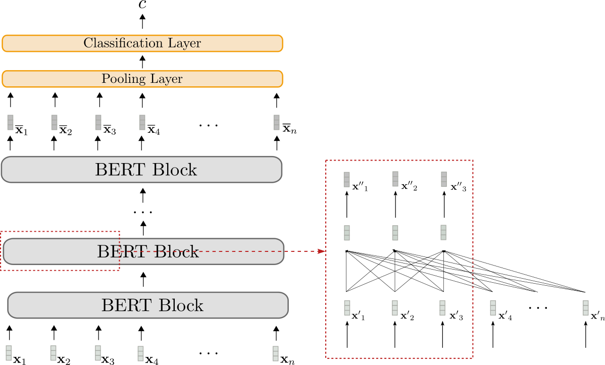
BERT 模型顯示為灰色。該模型堆疊了多個BERT 塊,每個塊由雙向自注意力層(紅色框下部所示)和兩個前饋層(紅色框上部所示)組成。
每個 BERT 塊都利用**雙向**自注意力來處理輸入序列 (淺灰色所示),以生成更“精煉”的語境化輸出序列 (略深灰色所示)。最後一個 BERT 塊的語境化輸出序列,即 ,可以透過新增一個任務特定的分類層(橙色所示),如上所述,對映到單個輸出類別 。
僅編碼器模型只能將輸入序列對映到先驗已知輸出長度的輸出序列。總之,輸出維度不依賴於輸入序列,這使得使用僅編碼器模型進行序列到序列任務具有不利和不切實際的缺點。
正如所有僅編碼器模型一樣,BERT 的架構與編碼器-解碼器筆記本中“編碼器”部分所示的基於 Transformer 的編碼器-解碼器模型的編碼器部分架構完全對應。
GPT2
GPT2 是一個僅解碼器模型,它利用單向(即“因果”)自注意力,將輸入序列 對映到“下一個詞”的 logits 向量序列
透過對 logits 向量 應用 softmax 操作,模型可以定義詞序列 的機率分佈。具體來說,詞序列 的機率分佈可以分解為 個條件“下一個詞”分佈
表示給定所有先前的詞 後,下一個詞 的機率分佈,並定義為對 logits 向量 應用 softmax 操作。總而言之,以下等式成立。
有關更多詳細資訊,請參閱編碼器-解碼器部落格文章的解碼器部分。
現在也讓我們視覺化 GPT2。
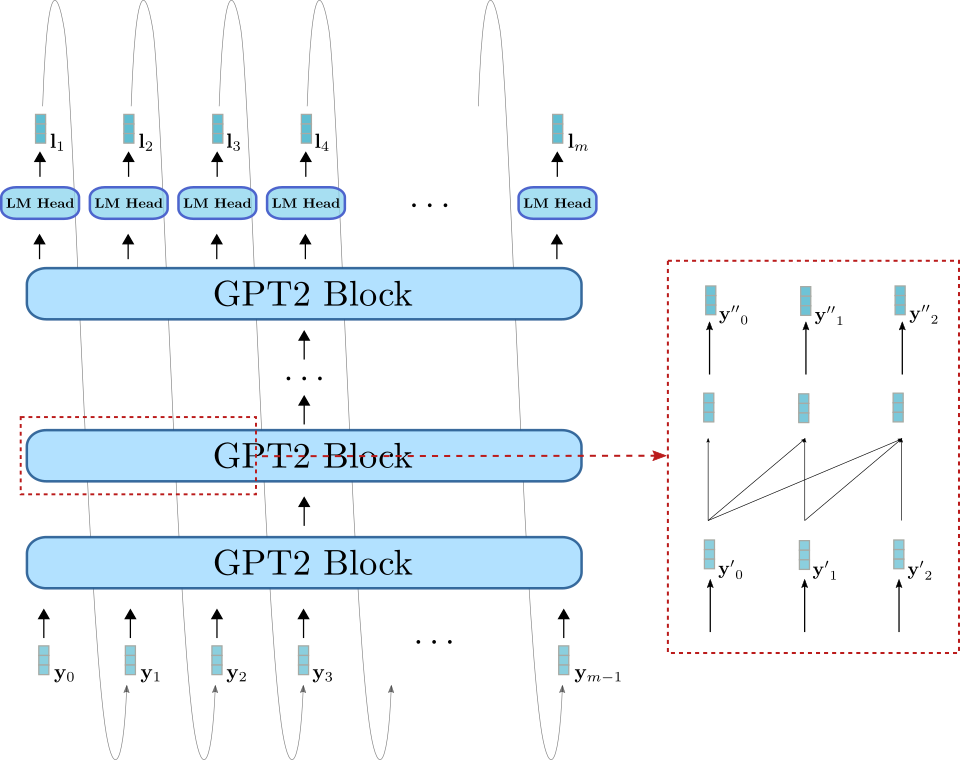
與BERT類似,GPT2由一系列*GPT2塊*組成。與BERT塊不同,GPT2塊利用**單向**自注意力機制處理一些輸入向量 (右下方淺藍色所示),將其處理成輸出向量序列 (右上方深藍色所示)。除了GPT2塊堆疊外,該模型還有一個線性層,稱為*LM Head*,它將最後一個GPT2塊的輸出向量對映到logits向量。如前所述,logits向量可以用於取樣新的輸入向量。
GPT2主要用於*開放域*文字生成。首先,將輸入提示輸入到模型中,以獲得條件分佈。然後從該分佈中取樣下一個詞(上圖中灰色箭頭所示),並將其新增到輸入中。以自迴歸的方式,詞可以從中取樣,以此類推。
因此,GPT2非常適合*語言生成*,但不太適合*條件*生成。透過將輸入提示設定為等於序列輸入,GPT2可以很好地用於條件生成。然而,與編碼器-解碼器架構相比,該模型架構存在根本性缺陷,如Raffel et al. (2019)第17頁所解釋。簡而言之,單向自注意力強制模型對序列輸入的表示受到不必要的限制,因為不能依賴於。
編碼器-解碼器
由於*僅編碼器*模型需要*預先*知道輸出長度,因此它們似乎不適用於序列到序列任務。*僅解碼器*模型可以很好地用於序列到序列任務,但也如上所述存在某些架構限制。
當前處理*序列到序列*任務的主要方法是*基於Transformer*的**編碼器-解碼器**模型——通常也稱為*seq2seq Transformer*模型。編碼器-解碼器模型由Vaswani et al. (2017)引入,此後已被證明在*序列到序列*任務上的表現優於獨立語言模型(即僅解碼器模型),例如Raffel et al. (2020)。本質上,編碼器-解碼器模型是*獨立*編碼器(如BERT)和*獨立*解碼器模型(如GPT2)的組合。有關基於Transformer的編碼器-解碼器模型的具體架構的更多詳細資訊,請參閱這篇部落格文章。
現在,我們知道大型預訓練*獨立*編碼器和解碼器模型的自由可用檢查點(例如*BERT*和*GPT*)可以提高許多NLU任務的效能並降低訓練成本。我們也知道編碼器-解碼器模型本質上是*獨立*編碼器和解碼器模型的組合。這自然引出了一個問題:如何利用獨立模型檢查點用於編碼器-解碼器模型,以及哪些模型組合在某些*序列到序列*任務上表現最佳。
2020年,Sascha Rothe、Shashi Narayan和Aliaksei Severyn在他們的論文**利用預訓練檢查點進行序列生成任務**中精確地研究了這個問題。該論文對不同的編碼器-解碼器模型組合和微調技術進行了精彩分析,我們將在後面更詳細地研究。
從預訓練的獨立模型檢查點構建編碼器-解碼器模型被定義為對編碼器-解碼器模型進行*熱啟動*。以下各節將展示熱啟動編碼器-解碼器模型的理論工作原理、如何使用🤗Transformers將理論付諸實踐,並提供提高效能的實用技巧。
*預訓練語言模型*定義為神經網路
- 在*未標記*文字資料上進行訓練,即以任務無關的無監督方式進行訓練,並且
- 將輸入詞序列處理成*上下文相關*的嵌入。例如,Mikolov et al. (2013)的*連續詞袋*和*跳字圖*模型不被視為預訓練語言模型,因為它們的嵌入是上下文無關的。
*微調*被定義為使用預訓練語言模型的權重初始化的模型進行*任務特定*訓練。
輸入向量對應於預測第一個輸出詞所需的嵌入向量。
在不失一般性的前提下,我們排除歸一化層,以免使方程和插圖過於繁瑣。
有關單向自注意力如何用於“僅解碼器”模型(如GPT2)以及取樣如何精確工作的更多詳細資訊,請參閱編碼器-解碼器部落格文章的解碼器部分。
熱啟動編碼器-解碼器模型(理論)
閱讀了引言後,我們現在熟悉了*僅編碼器*和*僅解碼器*模型。我們注意到編碼器-解碼器模型架構本質上是*獨立*編碼器模型和*獨立*解碼器模型的組合,這引導我們思考如何從*獨立*模型檢查點*熱啟動*編碼器-解碼器模型。
有多種可能性可以熱啟動編碼器-解碼器模型。可以
- 從*僅編碼器*模型檢查點初始化編碼器和解碼器部分,例如BERT,
- 從*僅編碼器*模型檢查點初始化編碼器部分,例如BERT,並從*僅解碼器*檢查點初始化解碼器部分,例如GPT2,
- 僅使用*僅編碼器*模型檢查點初始化編碼器部分,或
- 僅使用*僅解碼器*模型檢查點初始化解碼器部分。
在下文中,我們將重點放在可能性1和2上。在理解了前兩種可能性之後,可能性3和4就變得微不足道了。
編碼器-解碼器模型回顧
首先,讓我們快速回顧一下編碼器-解碼器架構。
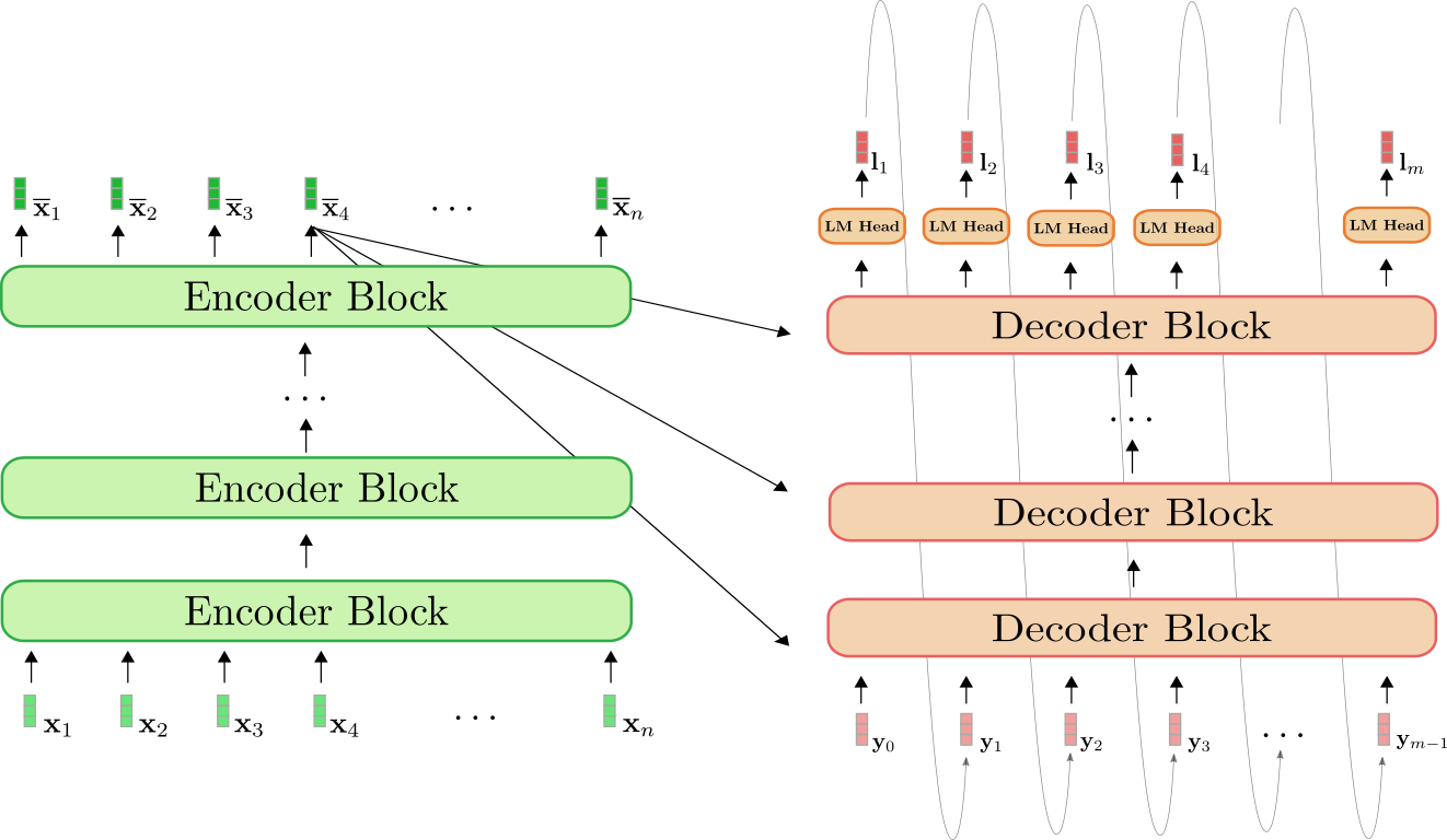
編碼器(綠色所示)是*編碼器塊*的堆疊。每個編碼器塊由一個*雙向自注意力*層和兩個前饋層組成。解碼器(橙色所示)是*解碼器塊*的堆疊,後面是一個稱為*LM Head*的密集層。每個解碼器塊由一個*單向自注意力*層、一個*交叉注意力*層和兩個前饋層組成。
編碼器將輸入序列對映到上下文編碼序列,其方式與BERT完全相同。然後,解碼器將上下文編碼序列和目標序列對映到logits向量。與GPT2類似,logits然後透過*softmax*操作用於定義目標序列以輸入序列為條件的分佈。
用數學術語來說,首先,條件分佈透過貝葉斯規則分解為個下一個詞的條件分佈。
每個“下一個詞”的條件分佈由logits向量的*softmax*定義,如下所示。
更多詳情請參閱編碼器-解碼器notebook。
使用BERT熱啟動編碼器-解碼器
現在,讓我們演示如何使用預訓練的BERT模型熱啟動編碼器-解碼器模型。BERT的預訓練權重引數用於初始化編碼器的權重引數和解碼器的權重引數。為此,BERT的架構與編碼器的架構進行比較,編碼器中所有在BERT中也存在的層都將使用相應BERT層的預訓練權重引數進行初始化。編碼器中所有在BERT中不存在的層將簡單地隨機初始化其權重引數。
讓我們進行視覺化。
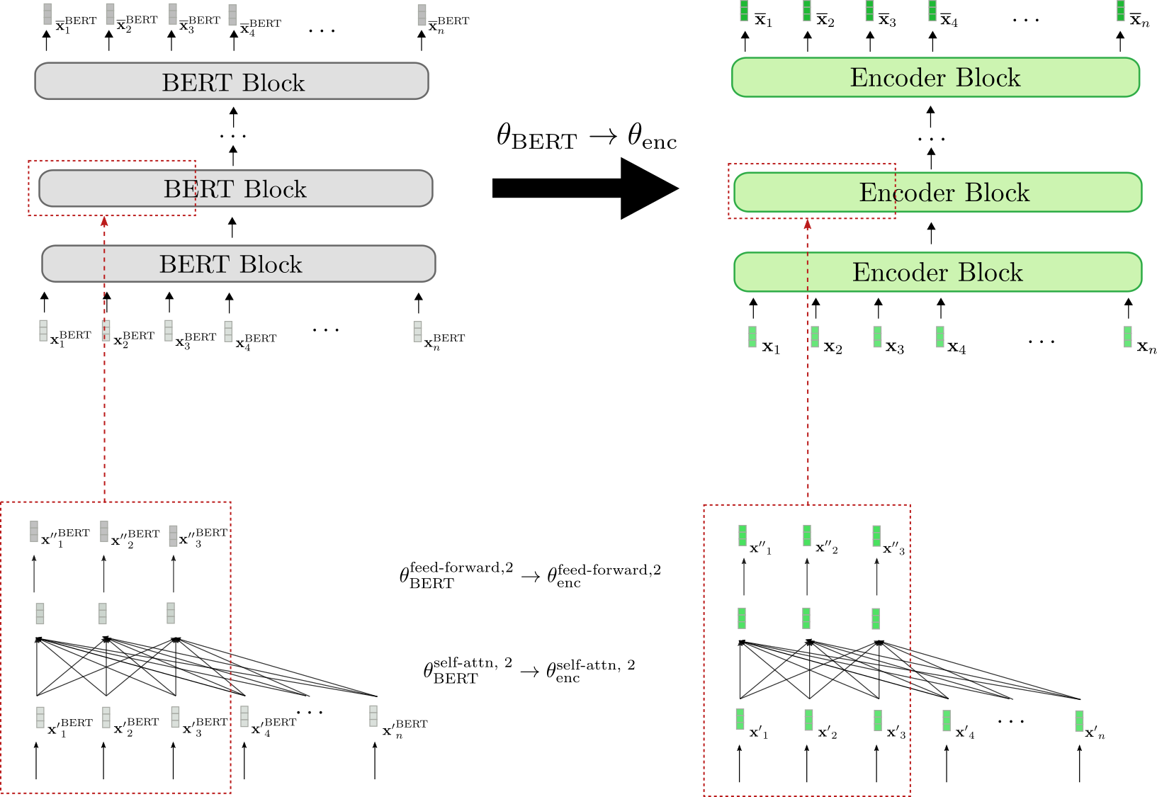
我們可以看到編碼器架構與BERT的架構一一對應。**所有**編碼器塊的*雙向自注意力層*和兩個*前饋層*的權重引數都使用相應BERT塊的權重引數進行初始化。這在第二個編碼器塊(底部紅色框)中得到了示例說明,其權重引數和在初始化時分別設定為BERT的權重引數和。
在微調之前,編碼器因此表現得與預訓練的 BERT 模型完全一樣。假設傳遞給編碼器的輸入序列 (綠色所示)等於傳遞給 BERT 的輸入序列 (灰色所示),這意味著相應的輸出向量序列 (深綠色所示)和 (深灰色所示)也必須相等。
接下來,我們來演示解碼器是如何進行熱啟動的。
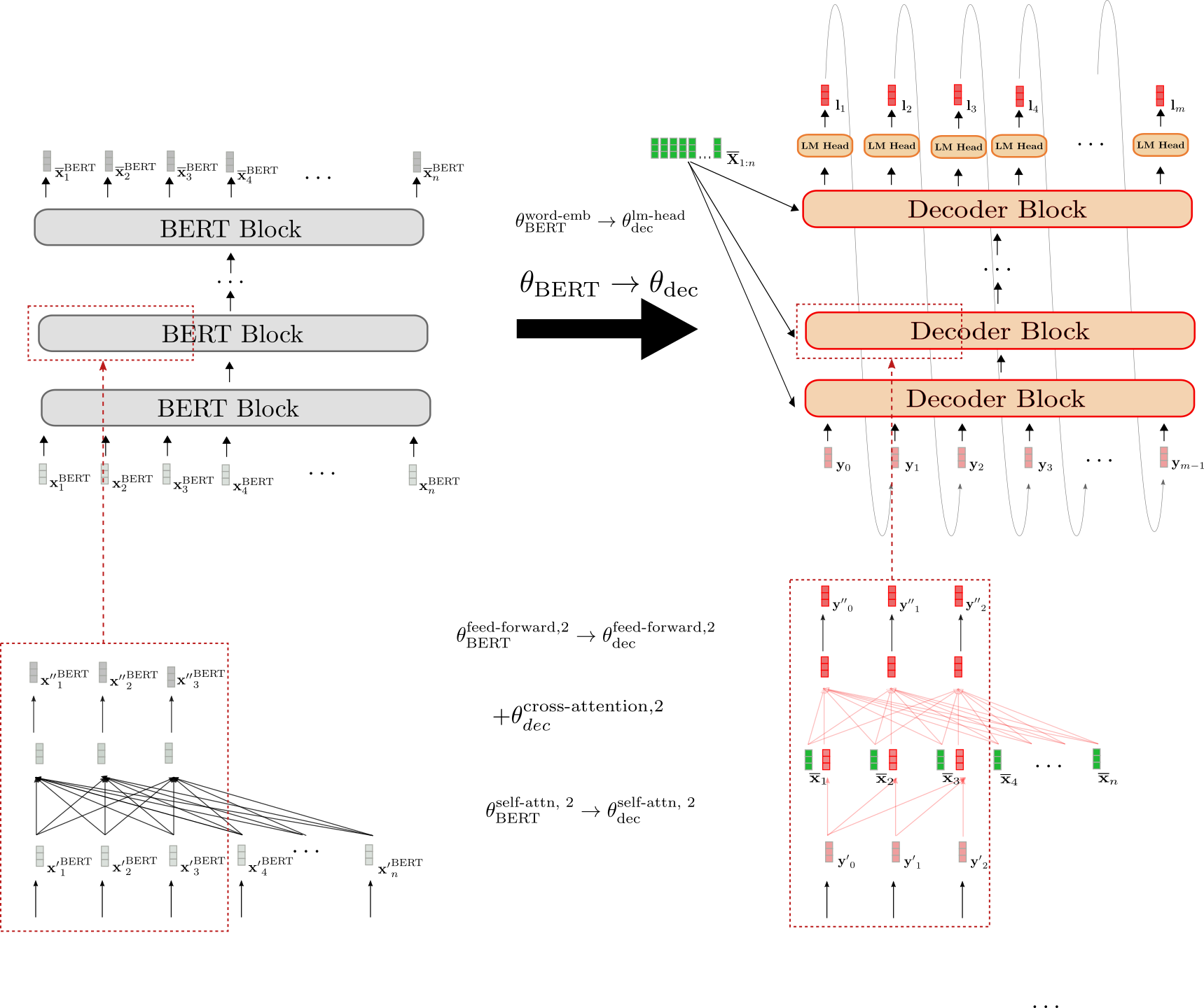
解碼器的架構與 BERT 的架構有三個不同之處。
首先,解碼器必須透過交叉注意力層以上下文編碼序列 為條件。因此,在每個 BERT 塊的自注意力層和兩個前饋層之間添加了隨機初始化的交叉注意力層。這在第二個塊中以 為例進行表示,並在右下方紅色框中以新增的紅色完全連線圖表示。這必然會改變每個修改過的 BERT 塊的行為,使得輸入向量(例如 )現在會產生隨機輸出向量 (由輸出向量 周圍的紅色邊框突出顯示)。
其次,BERT 的*雙向*自注意力層必須改為*單向*自注意力層,以符合自迴歸生成的要求。由於雙向和單向自注意力層都基於相同的*鍵*、*查詢*和*值*投影權重,因此解碼器的自注意力層權重可以用 BERT 的自注意力層權重進行初始化。例如,解碼器的單向自注意力層的查詢、鍵和值權重引數用 BERT 雙向自注意力層的相應引數進行初始化: 然而,在*單向*自注意力中,每個 token 只關注所有先前的 token,因此即使解碼器的自注意力層共享相同的權重,它們也會產生與 BERT 自注意力層不同的輸出向量。例如,比較右側框中解碼器的因果連線圖與左側框中 BERT 的完全連線圖。
第三,解碼器輸出一個 logit 向量序列 ,以便定義條件機率分佈 。因此,在最後一個解碼器塊的頂部添加了一個*LM Head*層。*LM Head*層的權重引數通常與詞嵌入 的權重引數相對應,因此不是隨機初始化的。這在頂部透過初始化 θdeclm-head 進行說明。
總而言之,當從預訓練的 BERT 模型熱啟動解碼器時,只有交叉注意力層權重是隨機初始化的。所有其他權重,包括自注意力層和 LM Head 的權重,都用 BERT 的預訓練權重引數進行初始化。
在熱啟動編碼器-解碼器模型後,權重將在*序列到序列*的下游任務(如摘要)上進行微調。
使用 BERT 和 GPT2 熱啟動編碼器-解碼器
我們可以不使用 BERT 檢查點熱啟動編碼器和解碼器,而是利用 BERT 檢查點用於編碼器,並利用 GPT2 檢查點用於解碼器。乍一看,一個僅包含解碼器的 GPT2 檢查點似乎更適合熱啟動解碼器,因為它已經過因果語言建模訓練,並且使用*單向*自注意力層。
讓我們演示如何使用 GPT2 檢查點來熱啟動解碼器。
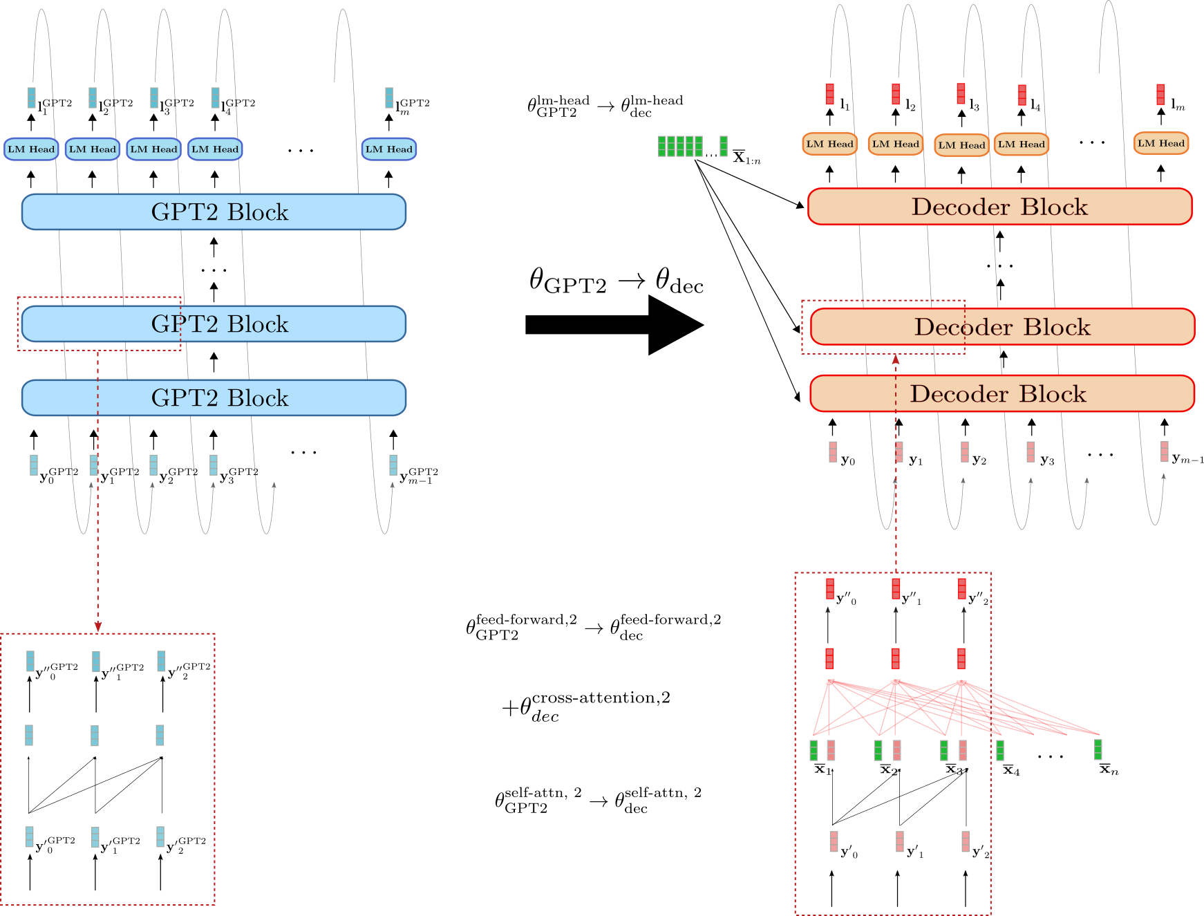
我們可以看到,解碼器與 GPT2 的相似度高於其與 BERT 的相似度。解碼器的*LM Head*的權重引數可以直接用 GPT2 的*LM Head*權重引數進行初始化,例如 。此外,解碼器和 GPT2 的塊都使用*單向*自注意力,因此假設輸入向量相同,解碼器自注意力層的輸出向量與 GPT2 的輸出向量等效,例如 y′0。與 BERT 初始化的解碼器相反,GPT2 初始化的解碼器因此保留了自注意力層的因果連線圖,如下方紅色框所示。
然而,GPT2 初始化的解碼器也必須以 為條件。因此,與 BERT 初始化的解碼器類似,為每個解碼器塊添加了隨機初始化的交叉注意力層權重引數。這以 為例進行說明。
儘管 GPT2 比 BERT 更像編碼器-解碼器模型中的解碼器部分,但由於每個解碼器塊中隨機初始化的交叉注意力層,GPT2 初始化的解碼器在不進行微調的情況下也會產生隨機的 logit 向量 。研究 GPT2 初始化的解碼器是否能產生更好的結果或更有效地進行微調將是很有趣的。
編碼器-解碼器權重共享
在 Raffel et al. (2020) 中,作者表明,一個隨機初始化的編碼器-解碼器模型,如果將編碼器的權重與解碼器共享,從而將記憶體佔用減少一半,其效能僅比其“不共享”版本略差。將編碼器的權重與解碼器共享意味著解碼器中與編碼器中相同位置的所有層共享相同的權重引數,即網路計算圖中的相同節點。
例如,第三個編碼器塊中自注意力層的查詢、鍵和值投影矩陣,定義為 、 和 ,與第三個解碼器塊中自注意力層的相應查詢、鍵和值投影矩陣 相同
=Wenc,kself-attn,3≡Wdec,kself-attn,3, =Wenc,qself-attn,3≡Wdec,qself-attn,3, =Wenc,vself-attn,3≡Wdec,vself-attn,3,
因此,鍵投影權重 ,Wvself-attn,3,Wqself-attn,3 在每次反向傳播過程中更新兩次——一次當梯度透過第三個解碼器塊反向傳播時,另一次當梯度透過第三個編碼器塊反向傳播時。
以同樣的方式,我們可以透過共享編碼器權重與解碼器來熱啟動編碼器-解碼器模型。為了在編碼器和解碼器之間共享權重,解碼器架構(不包括交叉注意力權重)需要與編碼器架構相同。因此,*編碼器-解碼器權重共享*僅在編碼器-解碼器模型從單個*僅編碼器*預訓練檢查點熱啟動時才相關。
太棒了!這就是關於熱啟動編碼器-解碼器模型的理論。現在讓我們看看一些結果。
不失一般性,我們排除了歸一化層,以免混淆方程式和插圖。 有關自注意力層如何運作的更多詳細資訊,請參閱變壓器編碼器-解碼器模型部落格文章的此部分(編碼器部分)和此部分(解碼器部分)。
熱啟動編碼器-解碼器模型(分析)
在本節中,我們將總結 Sascha Rothe、Shashi Narayan 和 Aliaksei Severyn 的《Leveraging Pre-trained Checkpoints for Sequence Generation Tasks》中提出的熱啟動編碼器-解碼器模型的研究結果。作者比較了熱啟動編碼器-解碼器模型與隨機初始化編碼器-解碼器模型在多個*序列到序列*任務(特別是*摘要*、*翻譯*、*句子拆分*和*句子合併*)上的效能。
更確切地說,公共可用的預訓練檢查點 BERT、RoBERTa 和 GPT2 以不同方式用於熱啟動編碼器-解碼器模型。例如,BERT 初始化的編碼器與 BERT 初始化的解碼器配對,生成 BERT2BERT 模型;或者 RoBERTa 初始化的編碼器與 GPT2 初始化的解碼器配對,生成 RoBERTa2GPT2 模型。此外,還研究了 RoBERTa 的編碼器和解碼器權重共享(如前一節所述)的效果,即 RoBERTaShare,以及 BERT 的效果,即 BERTShare。隨機或部分隨機初始化的編碼器-解碼器模型用作基線,例如完全隨機初始化的編碼器-解碼器模型(稱為 Rnd2Rnd)或 BERT 初始化的解碼器與隨機初始化的編碼器配對(定義為 Rnd2BERT)。
下表顯示了所有研究模型變體的完整列表,包括隨機初始化的權重數量(即“隨機”)和從各自預訓練檢查點初始化的權重數量(即“利用”)。所有模型均基於 12 層架構,隱藏尺寸嵌入為 768 維,對應於 🤗Transformers 模型中心的 `bert-base-cased`、`bert-base-uncased`、`roberta-base` 和 `gpt2` 檢查點。
| 模型 | 隨機 | 利用 | 總計 |
|---|---|---|---|
| Rnd2Rnd | 2.21 億 | 0 | 2.21 億 |
| Rnd2BERT | 1.12 億 | 1.09 億 | 2.21 億 |
| BERT2Rnd | 1.12 億 | 1.09 億 | 2.21 億 |
| Rnd2GPT2 | 1.14 億 | 1.25 億 | 2.38 億 |
| BERT2BERT | 2600 萬 | 1.95 億 | 2.21 億 |
| BERTShare | 2600 萬 | 1.09 億 | 1.35 億 |
| RoBERTaShare | 2600 萬 | 1.26 億 | 1.52 億 |
| BERT2GPT2 | 2600 萬 | 2.34 億 | 2.60 億 |
| RoBERTa2GPT2 | 2600 萬 | 2.50 億 | 2.76 億 |
基於 BERT2BERT 架構的模型*Rnd2Rnd*包含 2.21 億權重引數,所有這些引數都是隨機初始化的。另外兩個“基於 BERT”的基線*Rnd2BERT*和*BERT2Rnd*大約有一半的權重(即 1.12 億引數)是隨機初始化的。其餘的 1.09 億權重引數分別從預訓練的 `bert-base-uncased` 檢查點中提取,用於編碼器或解碼器部分。模型*BERT2BERT*、*BERT2GPT2*和*RoBERTa2GPT2*的所有編碼器權重引數都得到了利用(分別來自 `bert-base-uncased`、`roberta-base`),並且大部分解碼器權重引數也得到了利用(分別來自 `gpt2`、`bert-base-uncased`)。其中,2600 萬個解碼器權重引數(對應於 12 個交叉注意力層)是隨機初始化的。RoBERTa2GPT2 和 BERT2GPT2 與*Rnd2GPT2*基線進行了比較。此外,需要注意的是,共享模型變體*BERTShare*和*RoBERTaShare*的引數數量顯著減少,因為所有編碼器權重引數都與相應的解碼器權重引數共享。
實驗
上述模型在四個複雜程度遞增的序列到序列任務上進行了訓練和評估:句子級合併、句子級拆分、翻譯和抽象摘要。下表顯示了每個任務使用的資料集。
| 序列到序列任務 | 資料集 | 論文 | 🤗資料集 |
|---|---|---|---|
| 句子合併 | DiscoFuse | Geva et al. (2019) | 連結 |
| 句子拆分 | WikiSplit | Botha et al. (2018) | - |
| 翻譯 | WMT14 英語 => 德語 | Bojar et al. (2014) | 連結 |
| WMT14 德語 => 英語 | Bojar et al. (2014) | 連結 | |
| 抽象摘要 | CNN/Dailymail | Hermann et al. (2015) | 連結 |
| BBC XSum | Narayan et al. (2018a) | 連結 | |
| Gigaword | Napoles et al. (2012) | 連結 |
根據任務的不同,使用了略有不同的訓練方案。例如,根據資料集的大小和具體任務,訓練步數範圍為 20 萬到 50 萬,批處理大小設定為 128 或 256,輸入長度範圍為 128 到 512,輸出長度在 32 到 128 之間變化。然而,需要強調的是,在每個任務中,所有模型都使用相同的超引數進行訓練和評估,以確保公平比較。有關任務特定超引數設定的更多資訊,建議讀者參閱論文的*實驗*部分。
現在我們將簡要概述每個任務的結果。
句子合併和拆分(DiscoFuse、WikiSplit)
句子合併是將多個句子組合成一個連貫句子的任務。例如,以下兩個句子:
作為一名跑動阻擋者,蔡特勒的移動相對不錯。 蔡特勒在空間接觸點上經常掙扎。
應該用一個合適的*連線詞*連線起來,例如:
作為一名跑動阻擋者,蔡特勒的移動相對不錯。然而,他在空間接觸點上經常掙扎。
可以看出,“然而”這個連線詞為第一個句子到第二個句子提供了連貫的過渡。一個能夠生成這種連線詞的模型可以說已經學會推斷出上述兩個句子是相互對比的。
逆任務稱為句子拆分,包括將一個複雜的句子拆分成多個更簡單的句子,這些句子共同保留相同的含義。句子拆分被認為是文字簡化中的一項重要任務,參見Botha et al. (2018)。
例如,句子
《街頭霸王》是1989年為PC和Commodore 64釋出的系列兩款遊戲中的第一款
可以簡化為
《街頭霸王》是系列兩款遊戲中的第一款。它於1989年為PC和Commodore 64釋出
可以看出,長句試圖傳達兩個重要的資訊。一是這款遊戲是為PC釋出的系列兩款遊戲中的第一款,二是它釋出的年份。因此,句子拆分要求模型理解句子的哪個部分應該被分成兩個句子,這使得這項任務比句子合併更困難。
評估模型在句子合併和拆分任務上效能的常用指標是 SARI (Wu et al. (2016),它大致基於標籤和模型輸出的 F1 分數。
讓我們看看模型在句子合併和拆分上的表現。
| 模型 | 100% DiscoFuse (SARI) | 10% DiscoFuse (SARI) | 100% WikiSplit (SARI) |
|---|---|---|---|
| Rnd2Rnd | 86.9 | 81.5 | 61.7 |
| Rnd2BERT | 87.6 | 82.1 | 61.8 |
| BERT2Rnd | 89.3 | 86.1 | 63.1 |
| Rnd2GPT2 | 86.5 | 81.4 | 61.3 |
| BERT2BERT | 89.3 | 86.1 | 63.2 |
| BERTShare | 89.2 | 86.0 | 63.5 |
| RoBERTaShare | 89.7 | 86.0 | 63.4 |
| BERT2GPT2 | 88.4 | 84.1 | 62.4 |
| RoBERTa2GPT2 | 89.9 | 87.1 | 63.2 |
| --- | --- | --- | --- |
| RoBERTaShare (大型) | 90.3 | 87.7 | 63.8 |
前兩列顯示了編碼器-解碼器模型在 DiscoFuse 評估資料上的效能。第一列顯示了在所有 (100%) 訓練資料上訓練的編碼器-解碼器模型的結果,而第二列顯示了僅在 10% 訓練資料上訓練的模型的結果。我們觀察到,熱啟動模型比隨機初始化的基線模型 *Rnd2Rnd*、*Rnd2Bert* 和 *Rnd2GPT2* 表現顯著更好。僅在 10% 訓練資料上訓練的熱啟動 *RoBERTa2GPT2* 模型與在 100% 訓練資料上訓練的 *Rnd2Rnd* 模型效能相當。有趣的是,*Bert2Rnd* 基線模型的表現與完全熱啟動的 *Bert2Bert* 模型一樣好,這表明熱啟動編碼器部分比熱啟動解碼器部分更有效。最好的結果是由 *RoBERTa2GPT2* 獲得,其次是 *RobertaShare*。共享編碼器和解碼器權重引數似乎確實略微提高了模型的效能。
在更困難的句子拆分任務中,也出現了類似的模式。熱啟動編碼器-解碼器模型的效能顯著優於編碼器隨機初始化模型,並且具有共享權重引數的編碼器-解碼器模型比具有非耦合權重引數的模型產生更好的結果。在句子拆分任務上,BertShare 模型表現最佳,緊隨其後的是 RobertaShare。
除了12層模型變體,作者還訓練和評估了一個24層*RobertaShare (large)*模型,其效能顯著優於所有12層模型。
機器翻譯 (WMT14)
接下來,作者在機器翻譯 (MT) 中可能最常見的基準上評估了熱啟動的編碼器-解碼器模型——即 En De 和 De En WMT14 資料集。在本 Notebook 中,我們展示了 newstest2014 評估資料集的結果。因為該基準要求模型理解英語和德語詞彙,所以 BERT 初始化的編碼器-解碼器模型是從多語言預訓練檢查點 bert-base-multilingual-cased 熱啟動的。由於沒有公開可用的多語言 RoBERTa 檢查點,因此 MT 中排除了 RoBERTa 初始化的編碼器-解碼器模型。GPT2 初始化的模型像之前的實驗一樣從 gpt2 預訓練檢查點初始化。翻譯結果使用 BLUE-4 分數指標報告 。
| 模型 | 英 德 (BLEU-4) | 德 英 (BLEU-4) |
|---|---|---|
| Rnd2Rnd | 26.0 | 29.1 |
| Rnd2BERT | 27.2 | 30.4 |
| BERT2Rnd | 30.1 | 32.7 |
| Rnd2GPT2 | 19.6 | 23.2 |
| BERT2BERT | 30.1 | 32.7 |
| BERTShare | 29.6 | 32.6 |
| BERT2GPT2 | 23.2 | 31.4 |
| --- | --- | --- |
| BERT2Rnd (大型,自定義) | 31.7 | 34.2 |
| BERTShare (大型,自定義) | 30.5 | 33.8 |
我們再次觀察到,透過熱啟動編碼器部分,效能得到了顯著提升,其中 BERT2Rnd 和 BERT2BERT 在 En De 和 De En 任務上都取得了最佳結果。GPT2 初始化的模型在 En De 上的表現甚至明顯差於 Rnd2Rnd 基線。考慮到 gpt2 檢查點僅在英文文字上訓練,BERT2GPT2 和 Rnd2GPT2 模型在生成德語翻譯時遇到困難並不令人驚訝。這一假設得到了 BERT2GPT2 在 De En 任務上具有競爭力的結果(例如,31.4 對 32.7)的支援,因為 GPT2 的詞彙表適合英文輸出格式。與句子融合和句子拆分獲得的結果相反,共享編碼器和解碼器權重引數並未在機器翻譯中帶來效能提升。作者指出的可能原因包括
- MT 中編碼器-解碼器模型容量是一個重要因素,以及
- 編碼器和解碼器必須處理不同的語法和詞彙
由於 bert-base-multilingual-cased 檢查點在超過 100 種語言上進行了訓練,其詞彙量對於 En De 和 De En MT 可能不理想地過大。因此,作者在維基百科轉儲的英文和德文子集上預訓練了一個大型 BERT 僅編碼器檢查點,並隨後用它來熱啟動 BERT2Rnd 和 BERTShare 編碼器-解碼器模型。由於詞彙表的改進,觀察到了另一個顯著的效能提升,其中 BERT2Rnd (大型,自定義) 顯著優於所有其他模型。
摘要 (CNN/Dailymail, BBC XSum, Gigaword)
最後,編碼器-解碼器模型在可以說是最具挑戰性的序列到序列任務——摘要上進行了評估。作者選擇了三個具有不同特徵的摘要資料集進行評估:Gigaword (標題生成)、BBC XSum (極端摘要) 和 CNN/Dailymail (抽象摘要)。
Gigaword 資料集包含句子級別的抽象摘要,要求模型學習句子級別的理解、抽象和最終的轉述。Gigaword 中的典型資料樣本,例如
"*委內瑞拉總統烏戈·查韋斯週四表示,他已下令調查一起涉嫌涉及現役和退役軍官的政變陰謀。*",
將有一個相應的標題作為其標籤,例如
"查韋斯下令調查涉嫌政變陰謀"。
BBC XSum 資料集包含更長的文章式文字輸入,其標籤大多是單句摘要。該資料集要求模型不僅要學習文件級別的推理,還要學習高水平的抽象轉述。BBC XSUM 資料集的一些資料樣本可以在此處檢視。
對於 CNN/Dailymail 資料集,與 BBC XSum 資料集長度相似的文件必須摘要為要點式故事摘要。因此,標籤通常包含多個句子。除了文件級別的理解之外,CNN/Dailymail 資料集還要求模型善於複製最突出的資訊。一些示例可以在此處檢視。
模型使用 Rouge 指標進行評估,其中 Rouge-2 分數如下所示。
好的,讓我們看看結果。
| 模型 | CNN/Dailymail (Rouge-2) | BBC XSum (Rouge-2) | Gigaword (Rouge-2) |
|---|---|---|---|
| Rnd2Rnd | 14.00 | 10.23 | 18.71 |
| Rnd2BERT | 15.55 | 11.52 | 18.91 |
| BERT2Rnd | 17.76 | 15.83 | 19.26 |
| Rnd2GPT2 | 8.81 | 8.77 | 18.39 |
| BERT2BERT | 17.84 | 15.24 | 19.68 |
| BERTShare | 18.10 | 16.12 | 19.81 |
| RoBERTaShare | 18.95 | 17.50 | 19.70 |
| BERT2GPT2 | 4.96 | 8.37 | 18.23 |
| RoBERTa2GPT2 | 14.72 | 5.20 | 19.21 |
| --- | --- | --- | --- |
| RoBERTaShare (大型) | 18.91 | 18.79 | 19.78 |
我們再次觀察到,熱啟動編碼器部分與隨機初始化的編碼器模型相比有顯著的效能提升,這在文件級抽象任務(即 CNN/Dailymail 和 BBC XSum)中尤為明顯。這表明,需要高水平抽象的任務比僅需要句子級抽象的任務更能從預訓練的編碼器部分中受益。除了 Gigaword,基於 GPT2 的編碼器-解碼器模型似乎不適合摘要。
此外,共享編碼器-解碼器模型在摘要任務中表現最佳。RoBERTaShare 和 BERTShare 在所有資料集上都表現最佳,其中在 BBC XSum 資料集上的優勢尤為顯著,在該資料集上,RoBERTaShare (大型) 比 BERT2BERT 和 BERT2Rnd 高出約 3 個 Rouge-2 點,比 Rnd2Rnd 高出 8 個 Rouge-2 點以上。正如作者所說,“這可能是因為 BBC 摘要句子的分佈與文件中句子的分佈相似,而 Gigaword 標題和 CNN/DailyMail 要點摘要則不一定如此”。直觀地說,這意味著在 BBC XSum 中,編碼器處理的輸入句子與解碼器處理的單句摘要在結構上非常相似,即長度相同、詞語選擇相似、語法相似。
結論
好的,讓我們得出結論並嘗試提出一些實用技巧。
我們已經觀察到,在所有任務中,與隨機初始化編碼器的編碼器-解碼器模型相比,熱啟動編碼器部分能顯著提高效能。另一方面,熱啟動解碼器似乎不那麼重要,在大多數任務中,BERT2BERT 與 BERT2Rnd 相當。一個直觀的原因是,由於 BERT 或 RoBERTa 初始化的編碼器部分沒有任何隨機初始化的權重引數,因此編碼器可以充分利用 BERT 或 RoBERTa 預訓練檢查點所獲得的知識。相比之下,熱啟動的解碼器始終有部分權重引數是隨機初始化的,這可能使得有效利用用於初始化解碼器的檢查點所獲得的知識變得更加困難。
接下來,我們注意到共享編碼器和解碼器權重通常是有益的,特別是當目標分佈與輸入分佈相似時(例如 BBC XSum)。然而,對於目標資料分佈與輸入資料分佈差異更大的資料集,以及已知模型容量 在其中扮演重要角色的資料集,例如 WMT14,編碼器-解碼器權重共享似乎是不利的。
最後,我們看到預訓練的“獨立”檢查點的詞彙表與解決序列到序列任務所需的詞彙表非常重要。例如,一個熱啟動的 BERT2GPT2 編碼器-解碼器在 En De MT 上的表現會很差,因為 GPT2 是在英語上預訓練的,而目標語言是德語。與 BERT2BERT、BERTShared 和 RoBERTaShared 相比,BERT2GPT2、Rnd2GPT2 和 RoBERTa2GPT2 的整體表現不佳表明共享詞彙表更有效。此外,這表明用預訓練的 GPT2 檢查點初始化解碼器部分並不比用預訓練的 BERT 檢查點初始化它更有效,儘管 GPT2 在其架構上與解碼器更相似。
對於上述每個任務,效能最佳的模型已移植到 🤗Transformers,可在此處訪問
- RoBERTaShared (大型) - Wikisplit: google/roberta2roberta_L-24_wikisplit。
- RoBERTaShared (大型) - Discofuse: google/roberta2roberta_L-24_discofuse。
- BERT2BERT (大型) - WMT en de: google/bert2bert_L-24_wmt_en_de。
- BERT2BERT (大型) - WMT de en: google/bert2bert_L-24_wmt_de_en。
- RoBERTaShared (大型) - CNN/Dailymail: google/roberta2roberta_L-24_cnn_daily_mail。
- RoBERTaShared (大型) - BBC XSum: google/roberta2roberta_L-24_bbc。
- RoBERTaShared (大型) - Gigaword: google/roberta2roberta_L-24_gigaword。
為了獲取 BLEU-4 分數,使用了 Tensorflow 官方 Transformer 實現 https://github.com/tensorflow/models/tree master/official/nlp/transformer 中的指令碼。請注意,與 Vaswani 等人 (2017) 使用的 tensor2tensor/utils/ get_ende_bleu.sh 不同,該指令碼不拆分名詞複合詞,但在注意到預處理的訓練集只包含 ascii 引號後,將 utf-8 引號標準化為 ascii 引號。
模型容量是模型對複雜模式建模能力的非正式定義。有時也定義為模型從越來越多資料中學習的能力。模型容量通常透過可訓練引數的數量來衡量——引數越多,模型容量越高。
使用 🤗Transformers 熱啟動編碼器-解碼器模型(實踐)
我們已經解釋了熱啟動編碼器-解碼器模型的理論,分析了多個數據集上的實證結果,並得出了實際結論。現在,我們將透過一個完整的程式碼示例來演示如何熱啟動 BERT2BERT 模型,並將其在 CNN/Dailymail 摘要任務上進行微調。我們將利用 🤗datasets 和 🤗Transformers 庫。
此外,以下列表提供了本 Notebook 和其他關於熱啟動其他編碼器-解碼器模型組合的 Notebook 的精簡版本。
- 關於 CNN/Dailymail 上的 BERT2BERT(本 Notebook 的精簡版),請點選此處。
- 關於 BBC XSum 上的 RoBERTaShare,請點選此處。
- 關於 WMT14 En De 上的 BERT2Rnd,請點選此處。
- 關於 DiscoFuse 上的 RoBERTa2GPT2,請點選此處。
注意:本 Notebook 僅使用少量訓練、驗證和測試資料樣本進行演示。要對完整訓練資料進行編碼器-解碼器模型微調,使用者應根據註釋中突出顯示的內容相應地更改訓練和資料預處理引數。
資料預處理
本節將展示如何對資料進行預處理以進行訓練。更重要的是,我們試圖讓讀者對如何決定預處理資料的過程有一些瞭解。
我們將需要安裝 datasets 和 transformers。
!pip install datasets==1.0.2
!pip install transformers==4.2.1
讓我們首先下載 CNN/Dailymail 資料集。
import datasets
train_data = datasets.load_dataset("cnn_dailymail", "3.0.0", split="train")
好的,讓我們先對資料集有一個初步印象。另外,資料集也可以使用優秀的線上 datasets viewer 進行視覺化。
train_data.info.description
我們的輸入稱為 article,我們的標籤稱為 highlights。現在讓我們打印出訓練資料的第一個示例,以便對資料有一個感覺。
import pandas as pd
from IPython.display import display, HTML
from datasets import ClassLabel

df = pd.DataFrame(train_data[:1])
del df["id"]
for column, typ in train_data.features.items():
      if isinstance(typ, ClassLabel):
          df[column] = df[column].transform(lambda i: typ.names[i])
display(HTML(df.to_html()))
OUTPUT:
-------
Article:
"""It's official: U.S. President Barack Obama wants lawmakers to weigh in on whether to use military force in Syria. Obama sent a letter to the heads of the House and Senate on Saturday night, hours after announcing that he believes military action against Syrian targets is the right step to take over the alleged use of chemical weapons. The proposed legislation from Obama asks Congress to approve the use of military force "to deter, disrupt, prevent and degrade the potential for future uses of chemical weapons or other weapons of mass destruction." It's a step that is set to turn an international crisis into a fierce domestic political battle. There are key questions looming over the debate: What did U.N. weapons inspectors find in Syria? What happens if Congress votes no? And how will the Syrian government react? In a televised address from the White House Rose Garden earlier Saturday, the president said he would take his case to Congress, not because he has to -- but because he wants to. "While I believe I have the authority to carry out this military action without specific congressional authorization, I know that the country will be stronger if we take this course, and our actions will be even more effective," he said. "We should have this debate, because the issues are too big for business as usual." Obama said top congressional leaders had agreed to schedule a debate when the body returns to Washington on September 9. The Senate Foreign Relations Committee will hold a hearing over the matter on Tuesday, Sen. Robert Menendez said. Transcript: Read Obama's full remarks . Syrian crisis: Latest developments . U.N. inspectors leave Syria . Obama's remarks came shortly after U.N. inspectors left Syria, carrying evidence that will determine whether chemical weapons were used in an attack early last week in a Damascus suburb. "The aim of the game here, the mandate, is very clear -- and that is to ascertain whether chemical weapons were used -- and not by whom," U.N. spokesman Martin Nesirky told reporters on Saturday. But who used the weapons in the reported toxic gas attack in a Damascus suburb on August 21 has been a key point of global debate over the Syrian crisis. Top U.S. officials have said there's no doubt that the Syrian government was behind it, while Syrian officials have denied responsibility and blamed jihadists fighting with the rebels. British and U.S. intelligence reports say the attack involved chemical weapons, but U.N. officials have stressed the importance of waiting for an official report from inspectors. The inspectors will share their findings with U.N. Secretary-General Ban Ki-moon Ban, who has said he wants to wait until the U.N. team's final report is completed before presenting it to the U.N. Security Council. The Organization for the Prohibition of Chemical Weapons, which nine of the inspectors belong to, said Saturday that it could take up to three weeks to analyze the evidence they collected. "It needs time to be able to analyze the information and the samples," Nesirky said. He noted that Ban has repeatedly said there is no alternative to a political solution to the crisis in Syria, and that "a military solution is not an option." Bergen:  Syria is a problem from hell for the U.S. Obama: 'This menace must be confronted' Obama's senior advisers have debated the next steps to take, and the president's comments Saturday came amid mounting political pressure over the situation in Syria. Some U.S. lawmakers have called for immediate action while others warn of stepping into what could become a quagmire. Some global leaders have expressed support, but the British Parliament's vote against military action earlier this week was a blow to Obama's hopes of getting strong backing from key NATO allies. On Saturday, Obama proposed what he said would be a limited military action against Syrian President Bashar al-Assad. Any military attack would not be open-ended or include U.S. ground forces, he said. Syria's alleged use of chemical weapons earlier this month "is an assault on human dignity," the president said. A failure to respond with force, Obama argued,  "could lead to escalating use of chemical weapons or their proliferation to terrorist groups who would do our people harm. In a world with many dangers, this menace must be confronted." Syria missile strike: What would happen next? Map: U.S. and allied assets around Syria . Obama decision came Friday night . On Friday night, the president made a last-minute decision to consult lawmakers. What will happen if they vote no? It's unclear. A senior administration official told CNN that Obama has the authority to act without Congress -- even if Congress rejects his request for authorization to use force. Obama on Saturday continued to shore up support for a strike on the al-Assad government. He spoke by phone with French President Francois Hollande before his Rose Garden speech. "The two leaders agreed that the international community must deliver a resolute message to the Assad regime -- and others who would consider using chemical weapons -- that these crimes are unacceptable and those who violate this international norm will be held accountable by the world," the White House said. Meanwhile, as uncertainty loomed over how Congress would weigh in, U.S. military officials said they remained at the ready. 5 key assertions: U.S. intelligence report on Syria . Syria: Who wants what after chemical weapons horror . Reactions mixed to Obama's speech . A spokesman for the Syrian National Coalition said that the opposition group was disappointed by Obama's announcement. "Our fear now is that the lack of action could embolden the regime and they repeat his attacks in a more serious way," said spokesman Louay Safi. "So we are quite concerned." Some members of Congress applauded Obama's decision. House Speaker John Boehner, Majority Leader Eric Cantor, Majority Whip Kevin McCarthy and Conference Chair Cathy McMorris Rodgers issued a statement Saturday praising the president. "Under the Constitution, the responsibility to declare war lies with Congress," the Republican lawmakers said. "We are glad the president is seeking authorization for any military action in Syria in response to serious, substantive questions being raised." More than 160 legislators, including 63 of Obama's fellow Democrats, had signed letters calling for either a vote or at least a "full debate" before any U.S. action. British Prime Minister David Cameron, whose own attempt to get lawmakers in his country to support military action in Syria failed earlier this week, responded to Obama's speech in a Twitter post Saturday. "I understand and support Barack Obama's position on Syria," Cameron said. An influential lawmaker in Russia -- which has stood by Syria and criticized the United States -- had his own theory. "The main reason Obama is turning to the Congress:  the military operation did not get enough support either in the world, among allies of the US or in the United States itself," Alexei Pushkov, chairman of the international-affairs committee of the Russian State Duma, said in a Twitter post. In the United States, scattered groups of anti-war protesters around the country took to the streets Saturday. "Like many other Americans...we're just tired of the United States getting involved and invading and bombing other countries," said Robin Rosecrans, who was among hundreds at a Los Angeles demonstration. What do Syria's neighbors think? Why Russia, China, Iran stand by Assad . Syria's government unfazed . After Obama's speech, a military and political analyst on Syrian state TV said Obama is "embarrassed" that Russia opposes military action against Syria, is "crying for help" for someone to come to his rescue and is facing two defeats -- on the political and military levels. Syria's prime minister appeared unfazed by the saber-rattling. "The Syrian Army's status is on maximum readiness and fingers are on the trigger to confront all challenges," Wael Nader al-Halqi said during a meeting with a delegation of Syrian expatriates from Italy, according to a banner on Syria State TV that was broadcast prior to Obama's address. An anchor on Syrian state television said Obama "appeared to be preparing for an aggression on Syria based on repeated lies." A top Syrian diplomat told the state television network that Obama was facing pressure to take military action from Israel, Turkey, some Arabs and right-wing extremists in the United States. "I think he has done well by doing what Cameron did in terms of taking the issue to Parliament," said Bashar Jaafari, Syria's ambassador to the United Nations. Both Obama and Cameron, he said, "climbed to the top of the tree and don't know how to get down." The Syrian government has denied that it used chemical weapons in the August 21 attack, saying that jihadists fighting with the rebels used them in an effort to turn global sentiments against it. British intelligence had put the number of people killed in the attack at more than 350. On Saturday, Obama said "all told, well over 1,000 people were murdered." U.S. Secretary of State John Kerry on Friday cited a death toll of 1,429, more than 400 of them children. No explanation was offered for the discrepancy. Iran: U.S. military action in Syria would spark 'disaster' Opinion: Why strikes in Syria are a bad idea ."""
Summary:
"""Syrian official: Obama climbed to the top of the tree, "doesn't know how to get down"\nObama sends a letter to the heads of the House and Senate .\nObama to seek congressional approval on military action against Syria .\nAim is to determine whether CW were used, not by whom, says U.N. spokesman"""
輸入資料似乎由短新聞文章組成。有趣的是,標籤似乎是專案符號式的摘要。此時,應該檢視其他幾個示例,以便更好地瞭解資料。
這裡還應該注意到文字是區分大小寫的。這意味著如果我們想使用不區分大小寫的模型,我們必須小心。由於 CNN/Dailymail 是一個摘要資料集,模型將使用 ROUGE 指標進行評估。檢查 🤗datasets 中 ROUGE 的描述(參見此處),我們可以看到該指標是不區分大小寫的,這意味著在評估期間大寫字母將被規範化為小寫字母。因此,我們可以安全地利用不帶大小寫的檢查點,例如 bert-base-uncased。
太棒了!接下來,讓我們瞭解一下輸入資料和標籤的長度。
由於模型以token 長度計算長度,我們將使用 bert-base-uncased 分詞器來計算文章和摘要的長度。
首先,我們載入分詞器。
from transformers import BertTokenizerFast
tokenizer = BertTokenizerFast.from_pretrained("bert-base-uncased")
接下來,我們使用 .map() 來計算文章及其摘要的長度。由於我們知道 bert-base-uncased 可以處理的最大長度為 512,因此我們也對輸入樣本超過最大長度的百分比感興趣。同樣,我們計算摘要長度分別超過 64 和 128 的百分比。
我們可以將 .map() 函式定義如下。
# map article and summary len to dict as well as if sample is longer than 512 tokens
def map_to_length(x):
  x["article_len"] = len(tokenizer(x["article"]).input_ids)
  x["article_longer_512"] = int(x["article_len"] > 512)
  x["summary_len"] = len(tokenizer(x["highlights"]).input_ids)
  x["summary_longer_64"] = int(x["summary_len"] > 64)
  x["summary_longer_128"] = int(x["summary_len"] > 128)
  return x
檢視前 10000 個樣本就足夠了。我們可以透過使用 num_proc=4 的多個程序來加速對映。
sample_size = 10000
data_stats = train_data.select(range(sample_size)).map(map_to_length, num_proc=4)
計算出前 10000 個樣本的長度後,我們現在應該將它們平均。為此,我們可以使用 .map() 函式,並設定 batched=True 和 batch_size=-1,以便在 .map() 函式中訪問所有 10000 個樣本。
def compute_and_print_stats(x):
  if len(x["article_len"]) == sample_size:
    print(
        "Article Mean: {}, %-Articles > 512:{}, Summary Mean:{}, %-Summary > 64:{}, %-Summary > 128:{}".format(
            sum(x["article_len"]) / sample_size,
            sum(x["article_longer_512"]) / sample_size,
            sum(x["summary_len"]) / sample_size,
            sum(x["summary_longer_64"]) / sample_size,
            sum(x["summary_longer_128"]) / sample_size,
        )
    )

output = data_stats.map(
  compute_and_print_stats,
  batched=True,
  batch_size=-1,
)
    OUTPUT:
    -------
    Article Mean: 847.6216, %-Articles > 512:0.7355, Summary Mean:57.7742, %-Summary > 64:0.3185, %-Summary > 128:0.0
我們可以看到,一篇文章平均包含 848 個 token,其中約四分之三的文章長度超過了模型的 max_length 512。摘要平均長度為 57 個 token。我們 10000 個樣本的摘要中有超過 30% 的長度超過 64 個 token,但沒有一個長度超過 128 個 token。
bert-base-cased 限於 512 個 token,這意味著我們可能需要從文章中裁剪重要的資訊。由於大部分重要資訊通常出現在文章開頭,並且我們希望計算效率高,因此本 Notebook 決定堅持使用 bert-base-cased,其 max_length 為 512。這個選擇並非最優,但已在 CNN/Dailymail 上顯示出良好效果。或者,可以使用長程式列模型(如 Longformer)作為編碼器。
關於摘要長度,我們可以看到長度為 128 已經包含了所有摘要標籤。128 很容易在 bert-base-cased 的限制範圍內,因此我們決定將生成限制在 128。
我們再次使用 .map() 函式,這次是將每個訓練批次轉換為模型輸入批次。
“article”和“highlights”被分詞並分別準備為編碼器的“input_ids”和解碼器的“decoder_input_ids”。
“標籤”會自動向左移動,用於語言建模訓練。
最後,非常重要的是要記住忽略填充標籤的損失。在 🤗Transformers 中,可以透過將標籤設定為 -100 來完成此操作。好的,現在讓我們寫下對映函式。
encoder_max_length=512
decoder_max_length=128

def process_data_to_model_inputs(batch):
  # tokenize the inputs and labels
  inputs = tokenizer(batch["article"], padding="max_length", truncation=True, max_length=encoder_max_length)
  outputs = tokenizer(batch["highlights"], padding="max_length", truncation=True, max_length=decoder_max_length)

  batch["input_ids"] = inputs.input_ids
  batch["attention_mask"] = inputs.attention_mask
  batch["labels"] = outputs.input_ids.copy()

  # because BERT automatically shifts the labels, the labels correspond exactly to `decoder_input_ids`.
  # We have to make sure that the PAD token is ignored
  batch["labels"] = [[-100 if token == tokenizer.pad_token_id else token for token in labels] for labels in batch["labels"]]

  return batch
在本 Notebook 中,我們僅使用少量訓練示例來訓練和評估模型,並將 batch_size 設定為 4,以防止記憶體不足問題。
以下行將訓練資料減少到僅前 32 個示例。該單元格可以註釋掉或不執行,以進行完整的訓練執行。使用 16 的 batch_size 獲得了良好結果。
train_data = train_data.select(range(32))
好的,讓我們準備訓練資料。
# batch_size = 16
batch_size=4

train_data = train_data.map(
    process_data_to_model_inputs,
    batched=True,
    batch_size=batch_size,
    remove_columns=["article", "highlights", "id"]
)
檢視處理後的訓練資料集,我們可以看到列名 article、highlights 和 id 已被 EncoderDecoderModel 所需的引數替換。
train_data
OUTPUT:
-------
Dataset(features: {'attention_mask': Sequence(feature=Value(dtype='int64', id=None), length=-1, id=None), 'decoder_attention_mask': Sequence(feature=Value(dtype='int64', id=None), length=-1, id=None), 'decoder_input_ids': Sequence(feature=Value(dtype='int64', id=None), length=-1, id=None), 'input_ids': Sequence(feature=Value(dtype='int64', id=None), length=-1, id=None), 'labels': Sequence(feature=Value(dtype='int64', id=None), length=-1, id=None)}, num_rows: 32)
到目前為止,資料是使用 Python 的 List 格式進行操作的。讓我們將資料轉換為 PyTorch 張量,以便在 GPU 上進行訓練。
train_data.set_format(
    type="torch", columns=["input_ids", "attention_mask", "labels"],
)
太棒了,訓練資料的資料處理已經完成。類似地,我們可以對驗證資料做同樣的操作。
首先,我們載入 10% 的驗證資料集
val_data = datasets.load_dataset("cnn_dailymail", "3.0.0", split="validation[:10%]")
為了演示目的,驗證資料隨後減少到只有 8 個樣本,
val_data = val_data.select(range(8))
應用對映函式,
val_data = val_data.map(
    process_data_to_model_inputs,
    batched=True,
    batch_size=batch_size,
    remove_columns=["article", "highlights", "id"]
)
最後,驗證資料也被轉換為 PyTorch 張量。
val_data.set_format(
    type="torch", columns=["input_ids", "attention_mask", "labels"],
)
太好了!現在我們可以繼續熱啟動 EncoderDecoderModel。
熱啟動編碼器-解碼器模型
本節介紹如何使用 bert-base-cased 檢查點熱啟動編碼器-解碼器模型。
讓我們從匯入 EncoderDecoderModel 開始。有關 EncoderDecoderModel 類的更詳細資訊,建議讀者查閱文件。
from transformers import EncoderDecoderModel
與 🤗Transformers 中的其他模型類不同,EncoderDecoderModel 類有兩種載入預訓練權重的方法,即
“標準”
.from_pretrained(...)方法源自通用的PretrainedModel.from_pretrained(...)方法,因此與所有其他模型類完全相同。該函式需要一個模型識別符號,例如.from_pretrained("google/bert2bert_L-24_wmt_de_en"),並將單個.pt檢查點檔案載入到EncoderDecoderModel類中。一個特殊的
.from_encoder_decoder_pretrained(...)方法,可用於從兩個模型識別符號(一個用於編碼器,一個用於解碼器)熱啟動編碼器-解碼器模型。第一個模型識別符號用於透過AutoModel.from_pretrained(...)載入編碼器(參見文件此處),第二個模型識別符號用於透過AutoModelForCausalLM載入解碼器(參見文件此處)。
好的,讓我們熱啟動我們的 BERT2BERT 模型。如前所述,我們將使用 "bert-base-cased" 檢查點熱啟動編碼器和解碼器。
bert2bert = EncoderDecoderModel.from_encoder_decoder_pretrained("bert-base-uncased", "bert-base-uncased")
OUTPUT:
-------
"""Some weights of the model checkpoint at bert-base-uncased were not used when initializing BertLMHeadModel: ['cls.seq_relationship.weight', 'cls.seq_relationship.bias']
    - This IS expected if you are initializing BertLMHeadModel from the checkpoint of a model trained on another task or with another architecture (e.g. initializing a BertForSequenceClassification model from a BertForPretraining model).
    - This IS NOT expected if you are initializing BertLMHeadModel from the checkpoint of a model that you expect to be exactly identical (initializing a BertForSequenceClassification model from a BertForSequenceClassification model).
    Some weights of BertLMHeadModel were not initialized from the model checkpoint at bert-base-uncased and are newly initialized: ['bert.encoder.layer.0.crossattention.self.query.weight', 'bert.encoder.layer.0.crossattention.self.query.bias', 'bert.encoder.layer.0.crossattention.self.key.weight', 'bert.encoder.layer.0.crossattention.self.key.bias', 'bert.encoder.layer.0.crossattention.self.value.weight', 'bert.encoder.layer.0.crossattention.self.value.bias', 'bert.encoder.layer.0.crossattention.output.dense.weight', 'bert.encoder.layer.0.crossattention.output.dense.bias', 'bert.encoder.layer.0.crossattention.output.LayerNorm.weight', 'bert.encoder.layer.0.crossattention.output.LayerNorm.bias', 'bert.encoder.layer.1.crossattention.self.query.weight', 'bert.encoder.layer.1.crossattention.self.query.bias', 'bert.encoder.layer.1.crossattention.self.key.weight', 'bert.encoder.layer.1.crossattention.self.key.bias', 'bert.encoder.layer.1.crossattention.self.value.weight', 'bert.encoder.layer.1.crossattention.self.value.bias', 'bert.encoder.layer.1.crossattention.output.dense.weight', 'bert.encoder.layer.1.crossattention.output.dense.bias', 'bert.encoder.layer.1.crossattention.output.LayerNorm.weight', 'bert.encoder.layer.1.crossattention.output.LayerNorm.bias', 'bert.encoder.layer.2.crossattention.self.query.weight', 'bert.encoder.layer.2.crossattention.self.query.bias', 'bert.encoder.layer.2.crossattention.self.key.weight', 'bert.encoder.layer.2.crossattention.self.key.bias', 'bert.encoder.layer.2.crossattention.self.value.weight', 'bert.encoder.layer.2.crossattention.self.value.bias', 'bert.encoder.layer.2.crossattention.output.dense.weight', 'bert.encoder.layer.2.crossattention.output.dense.bias', 'bert.encoder.layer.2.crossattention.output.LayerNorm.weight', 'bert.encoder.layer.2.crossattention.output.LayerNorm.bias', 'bert.encoder.layer.3.crossattention.self.query.weight', 'bert.encoder.layer.3.crossattention.self.query.bias', 'bert.encoder.layer.3.crossattention.self.key.weight', 'bert.encoder.layer.3.crossattention.self.key.bias', 'bert.encoder.layer.3.crossattention.self.value.weight', 'bert.encoder.layer.3.crossattention.self.value.bias', 'bert.encoder.layer.3.crossattention.output.dense.weight', 'bert.encoder.layer.3.crossattention.output.dense.bias', 'bert.encoder.layer.3.crossattention.output.LayerNorm.weight', 'bert.encoder.layer.3.crossattention.output.LayerNorm.bias', 'bert.encoder.layer.4.crossattention.self.query.weight', 'bert.encoder.layer.4.crossattention.self.query.bias', 'bert.encoder.layer.4.crossattention.self.key.weight', 'bert.encoder.layer.4.crossattention.self.key.bias', 'bert.encoder.layer.4.crossattention.self.value.weight', 'bert.encoder.layer.4.crossattention.self.value.bias', 'bert.encoder.layer.4.crossattention.output.dense.weight', 'bert.encoder.layer.4.crossattention.output.dense.bias', 'bert.encoder.layer.4.crossattention.output.LayerNorm.weight', 'bert.encoder.layer.4.crossattention.output.LayerNorm.bias', 'bert.encoder.layer.5.crossattention.self.query.weight', 'bert.encoder.layer.5.crossattention.self.query.bias', 'bert.encoder.layer.5.crossattention.self.key.weight', 'bert.encoder.layer.5.crossattention.self.key.bias', 'bert.encoder.layer.5.crossattention.self.value.weight', 'bert.encoder.layer.5.crossattention.self.value.bias', 'bert.encoder.layer.5.crossattention.output.dense.weight', 'bert.encoder.layer.5.crossattention.output.dense.bias', 'bert.encoder.layer.5.crossattention.output.LayerNorm.weight', 'bert.encoder.layer.5.crossattention.output.LayerNorm.bias', 'bert.encoder.layer.6.crossattention.self.query.weight', 'bert.encoder.layer.6.crossattention.self.query.bias', 'bert.encoder.layer.6.crossattention.self.key.weight', 'bert.encoder.layer.6.crossattention.self.key.bias', 'bert.encoder.layer.6.crossattention.self.value.weight', 'bert.encoder.layer.6.crossattention.self.value.bias', 'bert.encoder.layer.6.crossattention.output.dense.weight', 'bert.encoder.layer.6.crossattention.output.dense.bias', 'bert.encoder.layer.6.crossattention.output.LayerNorm.weight', 'bert.encoder.layer.6.crossattention.output.LayerNorm.bias', 'bert.encoder.layer.7.crossattention.self.query.weight', 'bert.encoder.layer.7.crossattention.self.query.bias', 'bert.encoder.layer.7.crossattention.self.key.weight', 'bert.encoder.layer.7.crossattention.self.key.bias', 'bert.encoder.layer.7.crossattention.self.value.weight', 'bert.encoder.layer.7.crossattention.self.value.bias', 'bert.encoder.layer.7.crossattention.output.dense.weight', 'bert.encoder.layer.7.crossattention.output.dense.bias', 'bert.encoder.layer.7.crossattention.output.LayerNorm.weight', 'bert.encoder.layer.7.crossattention.output.LayerNorm.bias', 'bert.encoder.layer.8.crossattention.self.query.weight', 'bert.encoder.layer.8.crossattention.self.query.bias', 'bert.encoder.layer.8.crossattention.self.key.weight', 'bert.encoder.layer.8.crossattention.self.key.bias', 'bert.encoder.layer.8.crossattention.self.value.weight', 'bert.encoder.layer.8.crossattention.self.value.bias', 'bert.encoder.layer.8.crossattention.output.dense.weight', 'bert.encoder.layer.8.crossattention.output.dense.bias', 'bert.encoder.layer.8.crossattention.output.LayerNorm.weight', 'bert.encoder.layer.8.crossattention.output.LayerNorm.bias', 'bert.encoder.layer.9.crossattention.self.query.weight', 'bert.encoder.layer.9.crossattention.self.query.bias', 'bert.encoder.layer.9.crossattention.self.key.weight', 'bert.encoder.layer.9.crossattention.self.key.bias', 'bert.encoder.layer.9.crossattention.self.value.weight', 'bert.encoder.layer.9.crossattention.self.value.bias', 'bert.encoder.layer.9.crossattention.output.dense.weight', 'bert.encoder.layer.9.crossattention.output.dense.bias', 'bert.encoder.layer.9.crossattention.output.LayerNorm.weight', 'bert.encoder.layer.9.crossattention.output.LayerNorm.bias', 'bert.encoder.layer.10.crossattention.self.query.weight', 'bert.encoder.layer.10.crossattention.self.query.bias', 'bert.encoder.layer.10.crossattention.self.key.weight', 'bert.encoder.layer.10.crossattention.self.key.bias', 'bert.encoder.layer.10.crossattention.self.value.weight', 'bert.encoder.layer.10.crossattention.self.value.bias', 'bert.encoder.layer.10.crossattention.output.dense.weight', 'bert.encoder.layer.10.crossattention.output.dense.bias', 'bert.encoder.layer.10.crossattention.output.LayerNorm.weight', 'bert.encoder.layer.10.crossattention.output.LayerNorm.bias', 'bert.encoder.layer.11.crossattention.self.query.weight', 'bert.encoder.layer.11.crossattention.self.query.bias', 'bert.encoder.layer.11.crossattention.self.key.weight', 'bert.encoder.layer.11.crossattention.self.key.bias', 'bert.encoder.layer.11.crossattention.self.value.weight', 'bert.encoder.layer.11.crossattention.self.value.bias', 'bert.encoder.layer.11.crossattention.output.dense.weight', 'bert.encoder.layer.11.crossattention.output.dense.bias', 'bert.encoder.layer.11.crossattention.output.LayerNorm.weight', 'bert.encoder.layer.11.crossattention.output.LayerNorm.bias']"""
    You should probably TRAIN this model on a down-stream task to be able to use it for predictions and inference."""
我們應該仔細檢視這裡的警告。我們可以看到兩個與 "cls" 層對應的權重沒有被使用。這不應該是一個問題,因為我們不需要 BERT 的 CLS 層用於序列到序列任務。此外,我們注意到許多權重是“新”或隨機初始化的。仔細檢視這些權重,它們都對應於交叉注意力層,這正是我們閱讀了上述理論後所預期的。
讓我們仔細看看模型。
bert2bert
OUTPUT:
-------
    EncoderDecoderModel(
      (encoder): BertModel(
        (embeddings): BertEmbeddings(
          (word_embeddings): Embedding(30522, 768, padding_idx=0)
          (position_embeddings): Embedding(512, 768)
          (token_type_embeddings): Embedding(2, 768)
          (LayerNorm): LayerNorm((768,), eps=1e-12, elementwise_affine=True)
          (dropout): Dropout(p=0.1, inplace=False)
        )
        (encoder): BertEncoder(
          (layer): ModuleList(
            (0): BertLayer(
              (attention): BertAttention(
                (self): BertSelfAttention(
                  (query): Linear(in_features=768, out_features=768, bias=True)
                  (key): Linear(in_features=768, out_features=768, bias=True)
                  (value): Linear(in_features=768, out_features=768, bias=True)
                  (dropout): Dropout(p=0.1, inplace=False)
                )
                (output): BertSelfOutput(
                  (dense): Linear(in_features=768, out_features=768, bias=True)
                  (LayerNorm): LayerNorm((768,), eps=1e-12, elementwise_affine=True)
                  (dropout): Dropout(p=0.1, inplace=False)
                )
              )
              (intermediate): BertIntermediate(
                (dense): Linear(in_features=768, out_features=3072, bias=True)
              )
              (output): BertOutput(
                (dense): Linear(in_features=3072, out_features=768, bias=True)
                (LayerNorm): LayerNorm((768,), eps=1e-12, elementwise_affine=True)
                (dropout): Dropout(p=0.1, inplace=False)
              )
            ),
                        ...
                        ,
            (11): BertLayer(
              (attention): BertAttention(
                (self): BertSelfAttention(
                  (query): Linear(in_features=768, out_features=768, bias=True)
                  (key): Linear(in_features=768, out_features=768, bias=True)
                  (value): Linear(in_features=768, out_features=768, bias=True)
                  (dropout): Dropout(p=0.1, inplace=False)
                )
                (output): BertSelfOutput(
                  (dense): Linear(in_features=768, out_features=768, bias=True)
                  (LayerNorm): LayerNorm((768,), eps=1e-12, elementwise_affine=True)
                  (dropout): Dropout(p=0.1, inplace=False)
                )
              )
              (intermediate): BertIntermediate(
                (dense): Linear(in_features=768, out_features=3072, bias=True)
              )
              (output): BertOutput(
                (dense): Linear(in_features=3072, out_features=768, bias=True)
                (LayerNorm): LayerNorm((768,), eps=1e-12, elementwise_affine=True)
                (dropout): Dropout(p=0.1, inplace=False)
              )
            )
          )
        )
        (pooler): BertPooler(
          (dense): Linear(in_features=768, out_features=768, bias=True)
          (activation): Tanh()
        )
      )
      (decoder): BertLMHeadModel(
        (bert): BertModel(
          (embeddings): BertEmbeddings(
            (word_embeddings): Embedding(30522, 768, padding_idx=0)
            (position_embeddings): Embedding(512, 768)
            (token_type_embeddings): Embedding(2, 768)
            (LayerNorm): LayerNorm((768,), eps=1e-12, elementwise_affine=True)
            (dropout): Dropout(p=0.1, inplace=False)
          )
          (encoder): BertEncoder(
            (layer): ModuleList(
              (0): BertLayer(
                (attention): BertAttention(
                  (self): BertSelfAttention(
                    (query): Linear(in_features=768, out_features=768, bias=True)
                    (key): Linear(in_features=768, out_features=768, bias=True)
                    (value): Linear(in_features=768, out_features=768, bias=True)
                    (dropout): Dropout(p=0.1, inplace=False)
                  )
                  (output): BertSelfOutput(
                    (dense): Linear(in_features=768, out_features=768, bias=True)
                    (LayerNorm): LayerNorm((768,), eps=1e-12, elementwise_affine=True)
                    (dropout): Dropout(p=0.1, inplace=False)
                  )
                )
                (crossattention): BertAttention(
                  (self): BertSelfAttention(
                    (query): Linear(in_features=768, out_features=768, bias=True)
                    (key): Linear(in_features=768, out_features=768, bias=True)
                    (value): Linear(in_features=768, out_features=768, bias=True)
                    (dropout): Dropout(p=0.1, inplace=False)
                  )
                  (output): BertSelfOutput(
                    (dense): Linear(in_features=768, out_features=768, bias=True)
                    (LayerNorm): LayerNorm((768,), eps=1e-12, elementwise_affine=True)
                    (dropout): Dropout(p=0.1, inplace=False)
                  )
                )
                (intermediate): BertIntermediate(
                  (dense): Linear(in_features=768, out_features=3072, bias=True)
                )
                (output): BertOutput(
                  (dense): Linear(in_features=3072, out_features=768, bias=True)
                  (LayerNorm): LayerNorm((768,), eps=1e-12, elementwise_affine=True)
                  (dropout): Dropout(p=0.1, inplace=False)
                )
              ),
                            ...,
              (11): BertLayer(
                (attention): BertAttention(
                  (self): BertSelfAttention(
                    (query): Linear(in_features=768, out_features=768, bias=True)
                    (key): Linear(in_features=768, out_features=768, bias=True)
                    (value): Linear(in_features=768, out_features=768, bias=True)
                    (dropout): Dropout(p=0.1, inplace=False)
                  )
                  (output): BertSelfOutput(
                    (dense): Linear(in_features=768, out_features=768, bias=True)
                    (LayerNorm): LayerNorm((768,), eps=1e-12, elementwise_affine=True)
                    (dropout): Dropout(p=0.1, inplace=False)
                  )
                )
                (crossattention): BertAttention(
                  (self): BertSelfAttention(
                    (query): Linear(in_features=768, out_features=768, bias=True)
                    (key): Linear(in_features=768, out_features=768, bias=True)
                    (value): Linear(in_features=768, out_features=768, bias=True)
                    (dropout): Dropout(p=0.1, inplace=False)
                  )
                  (output): BertSelfOutput(
                    (dense): Linear(in_features=768, out_features=768, bias=True)
                    (LayerNorm): LayerNorm((768,), eps=1e-12, elementwise_affine=True)
                    (dropout): Dropout(p=0.1, inplace=False)
                  )
                )
                (intermediate): BertIntermediate(
                  (dense): Linear(in_features=768, out_features=3072, bias=True)
                )
                (output): BertOutput(
                  (dense): Linear(in_features=3072, out_features=768, bias=True)
                  (LayerNorm): LayerNorm((768,), eps=1e-12, elementwise_affine=True)
                  (dropout): Dropout(p=0.1, inplace=False)
                )
              )
            )
          )
        )
        (cls): BertOnlyMLMHead(
          (predictions): BertLMPredictionHead(
            (transform): BertPredictionHeadTransform(
              (dense): Linear(in_features=768, out_features=768, bias=True)
              (LayerNorm): LayerNorm((768,), eps=1e-12, elementwise_affine=True)
            )
            (decoder): Linear(in_features=768, out_features=30522, bias=True)
          )
        )
      )
    )
我們看到 bert2bert.encoder 是 BertModel 的例項,而 bert2bert.decoder 是 BertLMHeadModel 的例項。然而,這兩個例項現在被組合成一個單一的 torch.nn.Module,因此可以儲存為一個單一的 .pt 檢查點檔案。
讓我們嘗試使用標準 .save_pretrained(...) 方法。
bert2bert.save_pretrained("bert2bert")
同樣,模型可以使用標準的 .from_pretrained(...) 方法重新載入。
bert2bert = EncoderDecoderModel.from_pretrained("bert2bert")
太棒了。我們還要檢查配置。
bert2bert.config
OUTPUT:
-------
    EncoderDecoderConfig {
      "_name_or_path": "bert2bert",
      "architectures": [
        "EncoderDecoderModel"
      ],
      "decoder": {
        "_name_or_path": "bert-base-uncased",
        "add_cross_attention": true,
        "architectures": [
          "BertForMaskedLM"
        ],
        "attention_probs_dropout_prob": 0.1,
        "bad_words_ids": null,
        "bos_token_id": null,
        "chunk_size_feed_forward": 0,
        "decoder_start_token_id": null,
        "do_sample": false,
        "early_stopping": false,
        "eos_token_id": null,
        "finetuning_task": null,
        "gradient_checkpointing": false,
        "hidden_act": "gelu",
        "hidden_dropout_prob": 0.1,
        "hidden_size": 768,
        "id2label": {
          "0": "LABEL_0",
          "1": "LABEL_1"
        },
        "initializer_range": 0.02,
        "intermediate_size": 3072,
        "is_decoder": true,
        "is_encoder_decoder": false,
        "label2id": {
          "LABEL_0": 0,
          "LABEL_1": 1
        },
        "layer_norm_eps": 1e-12,
        "length_penalty": 1.0,
        "max_length": 20,
        "max_position_embeddings": 512,
        "min_length": 0,
        "model_type": "bert",
        "no_repeat_ngram_size": 0,
        "num_attention_heads": 12,
        "num_beams": 1,
        "num_hidden_layers": 12,
        "num_return_sequences": 1,
        "output_attentions": false,
        "output_hidden_states": false,
        "pad_token_id": 0,
        "prefix": null,
        "pruned_heads": {},
        "repetition_penalty": 1.0,
        "return_dict": false,
        "sep_token_id": null,
        "task_specific_params": null,
        "temperature": 1.0,
        "tie_encoder_decoder": false,
        "tie_word_embeddings": true,
        "tokenizer_class": null,
        "top_k": 50,
        "top_p": 1.0,
        "torchscript": false,
        "type_vocab_size": 2,
        "use_bfloat16": false,
        "use_cache": true,
        "vocab_size": 30522,
        "xla_device": null
      },
      "encoder": {
        "_name_or_path": "bert-base-uncased",
        "add_cross_attention": false,
        "architectures": [
          "BertForMaskedLM"
        ],
        "attention_probs_dropout_prob": 0.1,
        "bad_words_ids": null,
        "bos_token_id": null,
        "chunk_size_feed_forward": 0,
        "decoder_start_token_id": null,
        "do_sample": false,
        "early_stopping": false,
        "eos_token_id": null,
        "finetuning_task": null,
        "gradient_checkpointing": false,
        "hidden_act": "gelu",
        "hidden_dropout_prob": 0.1,
        "hidden_size": 768,
        "id2label": {
          "0": "LABEL_0",
          "1": "LABEL_1"
        },
        "initializer_range": 0.02,
        "intermediate_size": 3072,
        "is_decoder": false,
        "is_encoder_decoder": false,
        "label2id": {
          "LABEL_0": 0,
          "LABEL_1": 1
        },
        "layer_norm_eps": 1e-12,
        "length_penalty": 1.0,
        "max_length": 20,
        "max_position_embeddings": 512,
        "min_length": 0,
        "model_type": "bert",
        "no_repeat_ngram_size": 0,
        "num_attention_heads": 12,
        "num_beams": 1,
        "num_hidden_layers": 12,
        "num_return_sequences": 1,
        "output_attentions": false,
        "output_hidden_states": false,
        "pad_token_id": 0,
        "prefix": null,
        "pruned_heads": {},
        "repetition_penalty": 1.0,
        "return_dict": false,
        "sep_token_id": null,
        "task_specific_params": null,
        "temperature": 1.0,
        "tie_encoder_decoder": false,
        "tie_word_embeddings": true,
        "tokenizer_class": null,
        "top_k": 50,
        "top_p": 1.0,
        "torchscript": false,
        "type_vocab_size": 2,
        "use_bfloat16": false,
        "use_cache": true,
        "vocab_size": 30522,
        "xla_device": null
      },
      "is_encoder_decoder": true,
      "model_type": "encoder_decoder"
    }
該配置同樣由一個編碼器配置和一個解碼器配置組成,在我們的例子中,它們都是 BertConfig 的例項。然而,整個配置是 EncoderDecoderConfig 型別,因此它被儲存為一個單一的 .json 檔案。
總而言之,我們應該記住,一旦例項化了 EncoderDecoderModel 物件,它就提供了與 🤗Transformers 中任何其他編碼器-解碼器模型(例如 BART、T5、ProphetNet 等)相同的功能。唯一的區別是 EncoderDecoderModel 提供了額外的 from_encoder_decoder_pretrained(...) 函式,允許模型類從任意兩個編碼器和解碼器檢查點進行熱啟動。
此外,如果想建立一個共享的編碼器-解碼器模型,可以額外傳遞引數 tie_encoder_decoder=True,如下所示
shared_bert2bert = EncoderDecoderModel.from_encoder_decoder_pretrained("bert-base-cased", "bert-base-cased", tie_encoder_decoder=True)
作為比較,我們可以看到,正如預期的那樣,共享模型的引數要少得多。
print(f"\n\nNum Params. Shared: {shared_bert2bert.num_parameters()}, Non-Shared: {bert2bert.num_parameters()}")
OUTPUT:
-------
Num Params. Shared: 137298244, Non-Shared: 247363386
在本 Notebook 中,我們仍將訓練一個非共享的 Bert2Bert 模型,因此我們繼續使用 bert2bert 而不是 shared_bert2bert。
# free memory
del shared_bert2bert
我們已經熱啟動了一個 bert2bert 模型,但我們還沒有定義所有與束搜尋解碼相關的引數。
讓我們先設定特殊 token。bert-base-cased 沒有 decoder_start_token_id 或 eos_token_id,所以我們將分別使用它的 cls_token_id 和 sep_token_id。此外,我們應該在配置上定義一個 pad_token_id,並確保設定了正確的 vocab_size。
bert2bert.config.decoder_start_token_id = tokenizer.cls_token_id
bert2bert.config.eos_token_id = tokenizer.sep_token_id
bert2bert.config.pad_token_id = tokenizer.pad_token_id
bert2bert.config.vocab_size = bert2bert.config.encoder.vocab_size
接下來,讓我們定義所有與束搜尋解碼相關的引數。由於 bart-large-cnn 在 CNN/Dailymail 上表現良好,我們將直接複製其束搜尋解碼引數。
bert2bert.config.max_length = 142
bert2bert.config.min_length = 56
bert2bert.config.no_repeat_ngram_size = 3
bert2bert.config.early_stopping = True
bert2bert.config.length_penalty = 2.0
bert2bert.config.num_beams = 4
好的,現在讓我們開始微調熱啟動的 BERT2BERT 模型。
微調熱啟動編碼器-解碼器模型
本節將演示如何使用 Seq2SeqTrainer 微調熱啟動的編碼器-解碼器模型。
我們首先匯入 Seq2SeqTrainer 及其訓練引數 Seq2SeqTrainingArguments。
from transformers import Seq2SeqTrainer, Seq2SeqTrainingArguments
此外,我們需要一些 Python 包來使 Seq2SeqTrainer 工作。
!pip install git-python==1.0.3
!pip install rouge_score
!pip install sacrebleu
Seq2SeqTrainer 擴充套件了 🤗Transformer 的 Trainer,用於編碼器-解碼器模型。簡而言之,它允許在評估期間使用 generate(...) 函式,這對於驗證編碼器-解碼器模型在大多數序列到序列任務(如摘要)上的效能是必需的。
有關 Trainer 的更多資訊,請閱讀此簡短教程。
讓我們從配置 Seq2SeqTrainingArguments 開始。
引數 predict_with_generate 應設定為 True,這樣 Seq2SeqTrainer 就會在驗證資料上執行 generate(...) 函式,並將生成的輸出作為 predictions 傳遞給我們稍後將定義的 compute_metric(...) 函式。額外的引數派生自 TrainingArguments,可以在此處閱讀。對於完整的訓練執行,應根據需要更改這些引數。下面已註釋掉了一些不錯的預設值。
有關 Seq2SeqTrainer 的更多資訊,建議讀者查閱程式碼。
training_args = Seq2SeqTrainingArguments(
    predict_with_generate=True,
    evaluation_strategy="steps",
    per_device_train_batch_size=batch_size,
    per_device_eval_batch_size=batch_size,
    fp16=True,
    output_dir="./",
    logging_steps=2,
    save_steps=10,
    eval_steps=4,
    # logging_steps=1000,
    # save_steps=500,
    # eval_steps=7500,
    # warmup_steps=2000,
    # save_total_limit=3,
)
此外,我們需要定義一個函式來正確計算驗證期間的 ROUGE 分數。由於我們激活了 predict_with_generate,因此 compute_metrics(...) 函式需要使用 generate(...) 函式獲得的 predictions。與大多數摘要任務一樣,CNN/Dailymail 通常使用 ROUGE 分數進行評估。
首先,我們使用 🤗datasets 庫載入 ROUGE 指標。
rouge = datasets.load_metric("rouge")
接下來,我們將定義 compute_metrics(...) 函式。rouge 指標從兩個字串列表計算分數。因此,我們解碼 predictions 和 labels,確保 -100 被正確替換為 pad_token_id,並透過設定 skip_special_tokens=True 移除所有特殊字元。
def compute_metrics(pred):
    labels_ids = pred.label_ids
    pred_ids = pred.predictions

    pred_str = tokenizer.batch_decode(pred_ids, skip_special_tokens=True)
    labels_ids[labels_ids == -100] = tokenizer.pad_token_id
    label_str = tokenizer.batch_decode(labels_ids, skip_special_tokens=True)

    rouge_output = rouge.compute(predictions=pred_str, references=label_str, rouge_types=["rouge2"])["rouge2"].mid

    return {
        "rouge2_precision": round(rouge_output.precision, 4),
        "rouge2_recall": round(rouge_output.recall, 4),
        "rouge2_fmeasure": round(rouge_output.fmeasure, 4),
    }
太棒了,現在我們可以將所有引數傳遞給 Seq2SeqTrainer 並開始微調。執行以下單元格將需要大約 10 分鐘 ☕。
在完整的 CNN/Dailymail 訓練資料上微調 BERT2BERT 模型大約需要一臺 TITAN RTX GPU 8 小時。
# instantiate trainer
trainer = Seq2SeqTrainer(
    model=bert2bert,
    tokenizer=tokenizer,
    args=training_args,
    compute_metrics=compute_metrics,
    train_dataset=train_data,
    eval_dataset=val_data,
)
trainer.train()
太棒了,我們現在應該完全能夠微調熱啟動的編碼器-解碼器模型了。為了檢查微調結果,讓我們看看儲存的檢查點。
!ls
OUTPUT:
-------
    bert2bert      checkpoint-20  runs	   seq2seq_trainer.py
    checkpoint-10  __pycache__    sample_data  seq2seq_training_args.py
最後,我們可以像往常一樣透過 EncoderDecoderModel.from_pretrained(...) 方法載入檢查點。
dummy_bert2bert = EncoderDecoderModel.from_pretrained("./checkpoint-20")
評估
最後一步,我們可能希望在測試資料上評估 BERT2BERT 模型。
首先,我們不載入虛擬模型,而是載入一個在完整訓練資料集上微調過的 BERT2BERT 模型。此外,我們載入它的分詞器,它只是 bert-base-cased 分詞器的一個副本。
from transformers import BertTokenizer

bert2bert = EncoderDecoderModel.from_pretrained("patrickvonplaten/bert2bert_cnn_daily_mail").to("cuda")
tokenizer = BertTokenizer.from_pretrained("patrickvonplaten/bert2bert_cnn_daily_mail")
接下來,我們只加載 CNN/Dailymail 測試資料中的 2%。對於完整評估,顯然應該使用 100% 的資料。
test_data = datasets.load_dataset("cnn_dailymail", "3.0.0", split="test[:2%]")
現在,我們可以再次利用 🤗dataset 的便捷 map() 函式為每個測試樣本生成摘要。
對於每個資料樣本,我們
- 首先,對
"article"進行分詞, - 其次,生成輸出 token IDs,
- 第三,解碼輸出 token IDs 以獲得我們預測的摘要。
def generate_summary(batch):
    # cut off at BERT max length 512
    inputs = tokenizer(batch["article"], padding="max_length", truncation=True, max_length=512, return_tensors="pt")
    input_ids = inputs.input_ids.to("cuda")
    attention_mask = inputs.attention_mask.to("cuda")

    outputs = bert2bert.generate(input_ids, attention_mask=attention_mask)

    output_str = tokenizer.batch_decode(outputs, skip_special_tokens=True)

    batch["pred_summary"] = output_str

    return batch
讓我們執行 map 函式來獲取 results 字典,其中儲存了模型的每個樣本的預測摘要。執行以下單元格可能需要約 10 分鐘 ☕。
batch_size = 16  # change to 64 for full evaluation

results = test_data.map(generate_summary, batched=True, batch_size=batch_size, remove_columns=["article"])
最後,我們計算 ROUGE 分數。
rouge.compute(predictions=results["pred_summary"], references=results["highlights"], rouge_types=["rouge2"])["rouge2"].mid
OUTPUT:
-------
    Score(precision=0.10389454113300968, recall=0.1564771201053348, fmeasure=0.12175271663717585)
就是這樣。我們已經展示瞭如何熱啟動 BERT2BERT 模型並在 CNN/Dailymail 資料集上進行微調/評估。
完整訓練的 BERT2BERT 模型已上傳至 🤗模型中心,地址為 patrickvonplaten/bert2bert_cnn_daily_mail。
該模型在完整評估資料上取得了 18.22 的 ROUGE-2 分數,甚至比論文中報告的還要好一些。
有關一些摘要示例,建議讀者使用模型的線上推理 API,此處。
非常感謝 Google Research 的 Sascha Rothe、Shashi Narayan 和 Aliaksei Severyn,以及 🤗Hugging Face 的 Victor Sanh、Sylvain Gugger 和 Thomas Wolf 的校對和寶貴的反饋。