Diffusers 文件
Marigold 計算機視覺
並獲得增強的文件體驗
開始使用
Marigold 計算機視覺
Marigold 是一種基於擴散的方法,它包含一系列pipelines,專為稠密的計算機視覺任務設計,包括單目深度預測、表面法線估計和本徵影像分解。
本指南將引導您使用 Marigold 為影像和影片生成快速且高質量的預測。
每個 pipeline 都針對特定的計算機視覺任務量身定製,處理輸入的 RGB 影像並生成相應的預測。目前,已實現以下計算機視覺任務:
所有原始檢查點均在 Hugging Face 上的 PRS-ETH 組織下提供。它們設計用於 diffusers pipelines 和原始程式碼庫,後者也可用於訓練新的模型檢查點。以下是推薦檢查點的總結,所有這些檢查點在 1 到 4 步內都能產生可靠的結果。
| 模型權重 | 模態 | 評論 |
|---|---|---|
| prs-eth/marigold-depth-v1-1 | 深度 | 仿射不變深度預測為每個畫素分配一個介於 0(近平面)和 1(遠平面)之間的值,這兩個平面均由模型在推理過程中確定。 |
| prs-eth/marigold-normals-v0-1 | 法線 | 表面法線預測是螢幕空間相機中的單位長度三維向量,其值在 -1 到 1 的範圍內。 |
| prs-eth/marigold-iid-appearance-v1-1 | 本徵屬性 | InteriorVerse 分解由反照率和兩種 BRDF 材質屬性組成:粗糙度和金屬度。 |
| prs-eth/marigold-iid-lighting-v1-1 | 本徵屬性 | HyperSim 影像分解由反照率、漫反射陰影和非漫反射殘差:. |
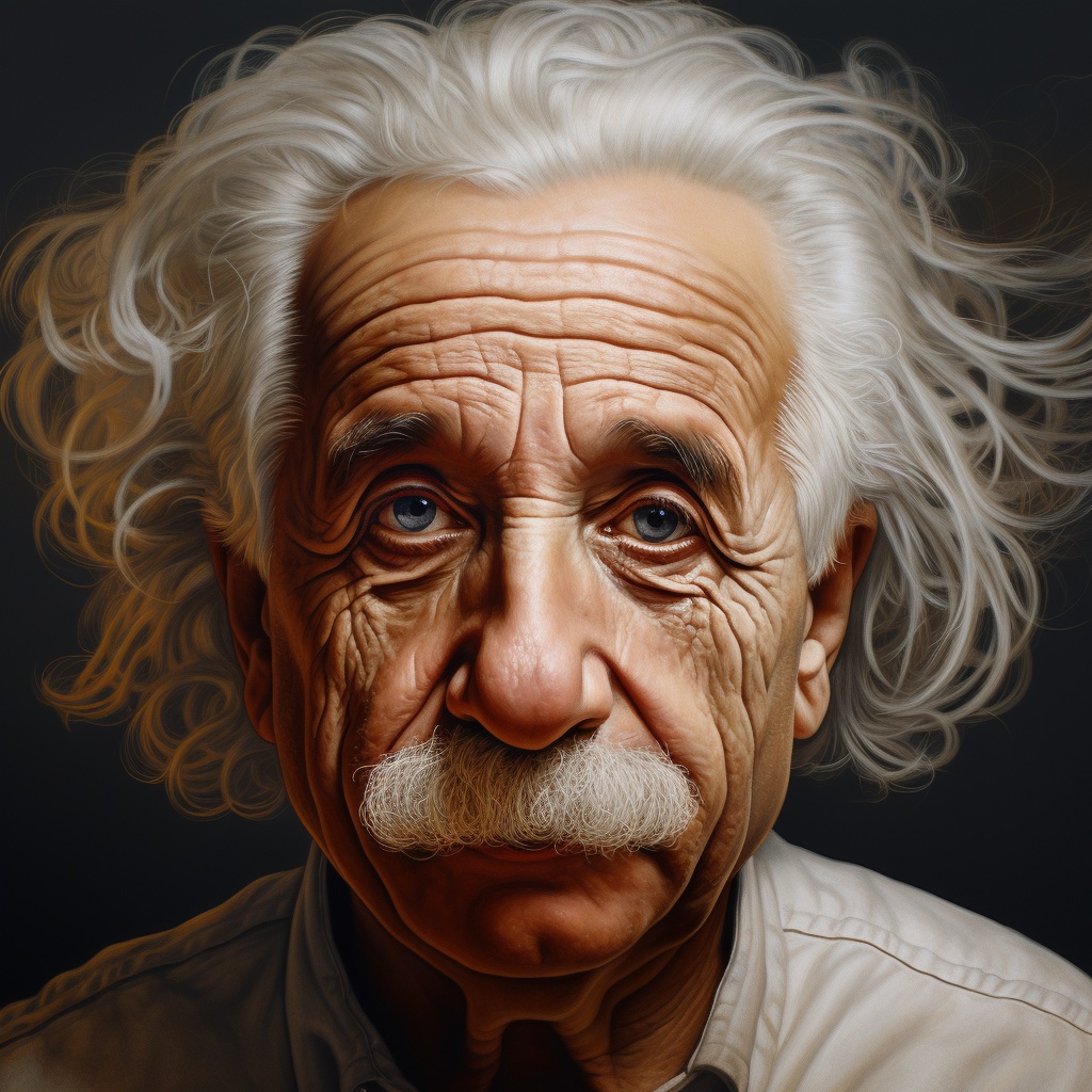
下面的示例主要針對深度預測,但它們可以普遍應用於其他支援的模態。我們使用由 Midjourney 生成的同一張阿爾伯特·愛因斯坦的輸入影像來展示預測結果。這使得比較不同模態和檢查點的預測視覺化變得更加容易。
深度預測
要獲得深度預測,請將 `prs-eth/marigold-depth-v1-1` 檢查點載入到 MarigoldDepthPipeline 中,將影像透過 pipeline 處理,然後儲存預測結果。
import diffusers
import torch

pipe = diffusers.MarigoldDepthPipeline.from_pretrained(
    "prs-eth/marigold-depth-v1-1", variant="fp16", torch_dtype=torch.float16
).to("cuda")

image = diffusers.utils.load_image("https://marigoldmonodepth.github.io/images/einstein.jpg")

depth = pipe(image)

vis = pipe.image_processor.visualize_depth(depth.prediction)
vis[0].save("einstein_depth.png")

depth_16bit = pipe.image_processor.export_depth_to_16bit_png(depth.prediction)
depth_16bit[0].save("einstein_depth_16bit.png")
visualize_depth() 函式應用 matplotlib 的顏色對映表 之一(預設為 `Spectral`),將預測的畫素值從單通道的 `[0, 1]` 深度範圍對映到 RGB 影像中。使用 `Spectral` 顏色對映表時,近深度的畫素被塗成紅色,遠深度的畫素被塗成藍色。16 位 PNG 檔案儲存了從 `[0, 1]` 範圍線性對映到 `[0, 65535]` 的單通道值。以下是原始預測和視覺化預測。在視覺化中,較暗和較近的區域(例如鬍鬚)更容易區分。


表面法線估計
將 `prs-eth/marigold-normals-v1-1` 檢查點載入到 MarigoldNormalsPipeline 中,將影像透過 pipeline 處理,然後儲存預測結果。
import diffusers
import torch

pipe = diffusers.MarigoldNormalsPipeline.from_pretrained(
    "prs-eth/marigold-normals-v1-1", variant="fp16", torch_dtype=torch.float16
).to("cuda")

image = diffusers.utils.load_image("https://marigoldmonodepth.github.io/images/einstein.jpg")

normals = pipe(image)

vis = pipe.image_processor.visualize_normals(normals.prediction)
vis[0].save("einstein_normals.png")
visualize_normals() 函式將畫素值在 `[-1, 1]` 範圍內的三維預測對映到 RGB 影像中。該視覺化函式支援翻轉表面法線座標軸,以使視覺化與其他參考系選擇相容。從概念上講,每個畫素根據參考系中的表面法線向量進行著色,其中 `X` 軸指向右,`Y` 軸指向上,`Z` 軸指向觀察者。以下是視覺化的預測結果:

在此示例中,鼻尖幾乎肯定有一個表面點,其表面法線向量直指觀察者,這意味著其座標為 `[0, 0, 1]`。該向量對映到 RGB `[128, 128, 255]`,對應於紫藍色。類似地,影像右側臉頰上的表面法線具有較大的 `X` 分量,這增加了紅色調。肩膀上指向上方的點具有較大的 `Y` 分量,這促進了綠色。
本徵影像分解
Marigold 為本徵影像分解(IID)提供了兩個模型:“外觀(Appearance)”和“光照(Lighting)”。每個模型都生成反照率圖,分別源自 InteriorVerse 和 Hypersim 的標註。
- “外觀”模型還估計材質屬性:粗糙度和金屬度。
- “光照”模型生成漫反射陰影和非漫反射殘差。
以下是儲存由“外觀”模型所做預測的示例程式碼:
import diffusers
import torch

pipe = diffusers.MarigoldIntrinsicsPipeline.from_pretrained(
    "prs-eth/marigold-iid-appearance-v1-1", variant="fp16", torch_dtype=torch.float16
).to("cuda")

image = diffusers.utils.load_image("https://marigoldmonodepth.github.io/images/einstein.jpg")

intrinsics = pipe(image)

vis = pipe.image_processor.visualize_intrinsics(intrinsics.prediction, pipe.target_properties)
vis[0]["albedo"].save("einstein_albedo.png")
vis[0]["roughness"].save("einstein_roughness.png")
vis[0]["metallicity"].save("einstein_metallicity.png")
另一個演示“光照”模型預測的示例:
import diffusers
import torch

pipe = diffusers.MarigoldIntrinsicsPipeline.from_pretrained(
    "prs-eth/marigold-iid-lighting-v1-1", variant="fp16", torch_dtype=torch.float16
).to("cuda")

image = diffusers.utils.load_image("https://marigoldmonodepth.github.io/images/einstein.jpg")

intrinsics = pipe(image)

vis = pipe.image_processor.visualize_intrinsics(intrinsics.prediction, pipe.target_properties)
vis[0]["albedo"].save("einstein_albedo.png")
vis[0]["shading"].save("einstein_shading.png")
vis[0]["residual"].save("einstein_residual.png")
兩種模型共享相同的 pipeline,同時支援不同的分解型別。確切的分解引數化(例如,sRGB 與線性空間)儲存在 `pipe.target_properties` 字典中,該字典被傳遞到 visualize_intrinsics() 函式中。
以下是一些展示預測分解輸出的示例。所有模態都可以在本徵影像分解 Space 中進行檢查。


加速推理
以上快速入門程式碼片段已經針對質量和速度進行了最佳化,載入了檢查點,利用了 `fp16` 版本的權重和計算,並執行了預設數量(4)的去噪擴散步驟。加速推理的第一步是以犧牲預測質量為代價,將去噪擴散步驟減少到最小值:
  import diffusers
  import torch

  pipe = diffusers.MarigoldDepthPipeline.from_pretrained(
      "prs-eth/marigold-depth-v1-1", variant="fp16", torch_dtype=torch.float16
  ).to("cuda")

  image = diffusers.utils.load_image("https://marigoldmonodepth.github.io/images/einstein.jpg")

- depth = pipe(image)
+ depth = pipe(image, num_inference_steps=1)
透過此更改,在 RTX 3090 GPU 上,`pipe` 呼叫在 280 毫秒內完成。在內部,輸入影像首先使用 Stable Diffusion VAE 編碼器進行編碼,然後由 U-Net 執行單個去噪步驟。最後,預測的潛變數透過 VAE 解碼器解碼到畫素空間。在這種設定中,三個模組呼叫中有兩個專用於在畫素和 LDM 的潛空間之間進行轉換。由於 Marigold 的潛空間與 Stable Diffusion 2.0 相容,透過使用輕量級的 SD VAE 替代品,推理速度可以提高 3 倍以上,將 RTX 3090 上的呼叫時間減少到 85 毫秒。請注意,使用輕量級 VAE 可能會略微降低預測的視覺質量。
  import diffusers
  import torch

  pipe = diffusers.MarigoldDepthPipeline.from_pretrained(
      "prs-eth/marigold-depth-v1-1", variant="fp16", torch_dtype=torch.float16
  ).to("cuda")

+ pipe.vae = diffusers.AutoencoderTiny.from_pretrained(
+     "madebyollin/taesd", torch_dtype=torch.float16
+ ).cuda()

  image = diffusers.utils.load_image("https://marigoldmonodepth.github.io/images/einstein.jpg")

  depth = pipe(image, num_inference_steps=1)
到目前為止,我們已經優化了擴散步驟和模型元件的數量。自注意力操作佔用了相當大一部分的計算量。可以透過使用更高效的注意力處理器來加速它們:
  import diffusers
  import torch
+ from diffusers.models.attention_processor import AttnProcessor2_0

  pipe = diffusers.MarigoldDepthPipeline.from_pretrained(
      "prs-eth/marigold-depth-v1-1", variant="fp16", torch_dtype=torch.float16
  ).to("cuda")

+ pipe.vae.set_attn_processor(AttnProcessor2_0())
+ pipe.unet.set_attn_processor(AttnProcessor2_0())

  image = diffusers.utils.load_image("https://marigoldmonodepth.github.io/images/einstein.jpg")

depth = pipe(image, num_inference_steps=1)最後,如最佳化中所建議,啟用 `torch.compile` 可以根據目標硬體進一步提升效能。然而,編譯在首次 pipeline 呼叫時會產生顯著的開銷,因此只有在重複呼叫同一 pipeline 例項時(例如在迴圈中)才會有益。
  import diffusers
  import torch
  from diffusers.models.attention_processor import AttnProcessor2_0

  pipe = diffusers.MarigoldDepthPipeline.from_pretrained(
      "prs-eth/marigold-depth-v1-1", variant="fp16", torch_dtype=torch.float16
  ).to("cuda")

  pipe.vae.set_attn_processor(AttnProcessor2_0())
  pipe.unet.set_attn_processor(AttnProcessor2_0())

+ pipe.vae = torch.compile(pipe.vae, mode="reduce-overhead", fullgraph=True)
+ pipe.unet = torch.compile(pipe.unet, mode="reduce-overhead", fullgraph=True)

  image = diffusers.utils.load_image("https://marigoldmonodepth.github.io/images/einstein.jpg")

  depth = pipe(image, num_inference_steps=1)
最大化精度和整合
Marigold pipelines 具有內建的整合機制,可以組合來自不同隨機潛變數的多個預測。這是一種透過暴力方式提高預測精度的方法,利用了擴散的生成特性。當 `ensemble_size` 引數設定為大於或等於 `3` 時,整合路徑會自動啟用。當目標是最大化精度時,同時調整 `num_inference_steps` 和 `ensemble_size` 是合理的。推薦值因檢查點而異,但主要取決於排程器型別。整合的效果在表面法線上尤其明顯:
  import diffusers

  pipe = diffusers.MarigoldNormalsPipeline.from_pretrained("prs-eth/marigold-normals-v1-1").to("cuda")

  image = diffusers.utils.load_image("https://marigoldmonodepth.github.io/images/einstein.jpg")

- depth = pipe(image)
+ depth = pipe(image, num_inference_steps=10, ensemble_size=5)

  vis = pipe.image_processor.visualize_normals(depth.prediction)
vis[0].save("einstein_normals.png") 
可以看出,所有具有精細結構(如頭髮)的區域都得到了更保守且平均更準確的預測。這樣的結果更適合對精度敏感的下游任務,例如三維重建。
具有時間一致性的逐幀影片處理
由於 Marigold 的生成特性,每個預測都是獨一無二的,並由用於潛變數初始化的隨機噪聲決定。與傳統的端到端稠密迴歸網路相比,這成了一個明顯的缺點,如下列影片所示:


為了解決這個問題,可以向 pipelines 傳遞 `latents` 引數,它定義了擴散的起始點。根據經驗,我們發現,將同一個起始點噪聲潛變數與對應於前一幀預測的潛變數進行凸組合,可以得到足夠平滑的結果,如下面的程式碼片段所示:
import imageio
import diffusers
import torch
from diffusers.models.attention_processor import AttnProcessor2_0
from PIL import Image
from tqdm import tqdm

device = "cuda"
path_in = "https://huggingface.co/spaces/prs-eth/marigold-lcm/resolve/c7adb5427947d2680944f898cd91d386bf0d4924/files/video/obama.mp4"
path_out = "obama_depth.gif"

pipe = diffusers.MarigoldDepthPipeline.from_pretrained(
    "prs-eth/marigold-depth-v1-1", variant="fp16", torch_dtype=torch.float16
).to(device)
pipe.vae = diffusers.AutoencoderTiny.from_pretrained(
    "madebyollin/taesd", torch_dtype=torch.float16
).to(device)
pipe.unet.set_attn_processor(AttnProcessor2_0())
pipe.vae = torch.compile(pipe.vae, mode="reduce-overhead", fullgraph=True)
pipe.unet = torch.compile(pipe.unet, mode="reduce-overhead", fullgraph=True)
pipe.set_progress_bar_config(disable=True)

with imageio.get_reader(path_in) as reader:
    size = reader.get_meta_data()['size']
    last_frame_latent = None
    latent_common = torch.randn(
        (1, 4, 768 * size[1] // (8 * max(size)), 768 * size[0] // (8 * max(size)))
    ).to(device=device, dtype=torch.float16)

    out = []
    for frame_id, frame in tqdm(enumerate(reader), desc="Processing Video"):
        frame = Image.fromarray(frame)
        latents = latent_common
        if last_frame_latent is not None:
            latents = 0.9 * latents + 0.1 * last_frame_latent

        depth = pipe(
            frame,
            num_inference_steps=1,
            match_input_resolution=False,
            latents=latents,
            output_latent=True,
        )
        last_frame_latent = depth.latent
        out.append(pipe.image_processor.visualize_depth(depth.prediction)[0])

    diffusers.utils.export_to_gif(out, path_out, fps=reader.get_meta_data()['fps'])
在這裡,擴散過程從給定的計算潛變數開始。pipeline 設定 `output_latent=True` 來訪問 `out.latent` 並計算其對下一幀潛變數初始化的貢獻。現在結果要穩定得多:

Marigold 用於 ControlNet
深度預測與擴散模型的一個非常常見的應用是與 ControlNet 結合使用。深度的清晰度在從 ControlNet 獲得高質量結果中起著至關重要的作用。如上與其他方法的比較所示,Marigold 在該任務上表現出色。下面的程式碼片段演示瞭如何載入影像、計算深度,並以相容的格式將其傳遞給 ControlNet:
import torch
import diffusers

device = "cuda"
generator = torch.Generator(device=device).manual_seed(2024)
image = diffusers.utils.load_image(
    "https://huggingface.co/datasets/huggingface/documentation-images/resolve/main/diffusers/controlnet_depth_source.png"
)

pipe = diffusers.MarigoldDepthPipeline.from_pretrained(
    "prs-eth/marigold-depth-v1-1", torch_dtype=torch.float16, variant="fp16"
).to(device)

depth_image = pipe(image, generator=generator).prediction
depth_image = pipe.image_processor.visualize_depth(depth_image, color_map="binary")
depth_image[0].save("motorcycle_controlnet_depth.png")

controlnet = diffusers.ControlNetModel.from_pretrained(
    "diffusers/controlnet-depth-sdxl-1.0", torch_dtype=torch.float16, variant="fp16"
).to(device)
pipe = diffusers.StableDiffusionXLControlNetPipeline.from_pretrained(
    "SG161222/RealVisXL_V4.0", torch_dtype=torch.float16, variant="fp16", controlnet=controlnet
).to(device)
pipe.scheduler = diffusers.DPMSolverMultistepScheduler.from_config(pipe.scheduler.config, use_karras_sigmas=True)

controlnet_out = pipe(
    prompt="high quality photo of a sports bike, city",
    negative_prompt="",
    guidance_scale=6.5,
    num_inference_steps=25,
    image=depth_image,
    controlnet_conditioning_scale=0.7,
    control_guidance_end=0.7,
    generator=generator,
).images
controlnet_out[0].save("motorcycle_controlnet_out.png")


定量評估
要對 Marigold 在標準排行榜和基準測試(如 NYU、KITTI 和其他資料集)中進行定量評估,請遵循論文中概述的評估協議:載入全精度 fp32 模型,併為 `num_inference_steps` 和 `ensemble_size` 使用適當的值。可選擇性地設定隨機種子以確保可復現性。最大化 `batch_size` 將實現最大的裝置利用率。
import diffusers
import torch

device = "cuda"
seed = 2024

generator = torch.Generator(device=device).manual_seed(seed)
pipe = diffusers.MarigoldDepthPipeline.from_pretrained("prs-eth/marigold-depth-v1-1").to(device)

image = diffusers.utils.load_image("https://marigoldmonodepth.github.io/images/einstein.jpg")

depth = pipe(
    image,
    num_inference_steps=4,  # set according to the evaluation protocol from the paper
    ensemble_size=10,       # set according to the evaluation protocol from the paper
    generator=generator,
)

# evaluate metrics
使用預測不確定性
Marigold pipelines 中內建的整合機制結合了從不同隨機潛變數獲得的多個預測。作為一個副作用,它可以用來量化認知(模型)不確定性;只需將 `ensemble_size` 指定為大於或等於 3,並設定 `output_uncertainty=True`。結果的不確定性將在輸出的 `uncertainty` 欄位中提供。它可以如下視覺化:
import diffusers
import torch

pipe = diffusers.MarigoldDepthPipeline.from_pretrained(
    "prs-eth/marigold-depth-v1-1", variant="fp16", torch_dtype=torch.float16
).to("cuda")

image = diffusers.utils.load_image("https://marigoldmonodepth.github.io/images/einstein.jpg")

depth = pipe(
	image,
	ensemble_size=10,  # any number >= 3
	output_uncertainty=True,
)

uncertainty = pipe.image_processor.visualize_uncertainty(depth.uncertainty)
uncertainty[0].save("einstein_depth_uncertainty.png")


不確定性的解釋很簡單:較高的值(白色)對應於模型難以做出一致預測的畫素。
- 深度模型在不連續處表現出最大的不確定性,即物體深度急劇變化的地方。
- 表面法線模型在像頭髮這樣的精細結構和像衣領區域這樣的黑暗區域中最不自信。
- 反照率不確定性表示為 RGB 影像,因為它獨立地捕捉每個顏色通道的不確定性,與深度和表面法線不同。它在陰影區域和不連續處也較高。
結論
我們希望 Marigold 對您的下游任務有所價值,無論是作為更廣泛的生成工作流程的一部分,還是用於基於感知的應用,如三維重建。
< > 在 GitHub 上更新