簡介

本 Notebook 將介紹如何使用 Stable Diffusion 透過現有 pipeline 來建立和修改影像的基礎知識。我們還將簡要介紹 pipeline 中的關鍵元件，而將更深入的探索留給深度剖析的 Notebook。具體來說，我們將涵蓋：

使用 StableDiffusionPipeline 從文字生成影像，並嘗試可用的引數
瞭解一些關鍵 pipeline 元件的實際作用
- VAE（變分自編碼器），它使這成為一個“潛在擴散模型”
- 處理文字提示的 tokenizer 和文字編碼器
- UNet 本身
- 排程器（scheduler），並探索不同的排程器
使用 pipeline 元件復現取樣迴圈
使用 Img2Img pipeline 編輯現有影像
使用 inpainting 和 Depth2Img pipeline

❓如果你有任何問題，請在 Hugging Face Discord 伺服器的 #diffusion-models-class 頻道中提出。如果你還沒有註冊，可以在這裡註冊：https://huggingface.co/join/discord

設定

%pip install -Uq diffusers ftfy accelerate

# Installing transformers from source for now since we need the latest version for Depth2Img
%pip install -Uq git+https://github.com/huggingface/transformers

import torch
import requests
from PIL import Image
from io import BytesIO
from matplotlib import pyplot as plt

# We'll be exploring a number of pipelines today!
from diffusers import (
    StableDiffusionPipeline,
    StableDiffusionImg2ImgPipeline,
    StableDiffusionInpaintPipeline,
    StableDiffusionDepth2ImgPipeline,
)


# We'll use a couple of demo images later in the notebook
def download_image(url):
    response = requests.get(url)
    return Image.open(BytesIO(response.content)).convert("RGB")


# Download images for inpainting example
img_url = "https://raw.githubusercontent.com/CompVis/latent-diffusion/main/data/inpainting_examples/overture-creations-5sI6fQgYIuo.png"
mask_url = "https://raw.githubusercontent.com/CompVis/latent-diffusion/main/data/inpainting_examples/overture-creations-5sI6fQgYIuo_mask.png"

img_height = 512
img_width = 512

init_image = download_image(img_url).resize((img_height, img_width))
mask_image = download_image(mask_url).resize((img_height, img_width))

# Set device
device = "mps" if torch.backends.mps.is_available() else "cuda" if torch.cuda.is_available() else "cpu"

從文字生成影像

讓我們載入一個 Stable Diffusion pipeline，看看它能做什麼。Stable Diffusion 有多個不同版本，在撰寫本文時最新的是 2.1 版本。如果你想探索舊版本，只需將模型 ID 替換為相應的模型（例如，你可以嘗試“CompVis/stable-diffusion-v1-4”或從 dreambooth 概念庫中選擇一個模型）。

# Load the pipeline
model_id = "stabilityai/stable-diffusion-2-1-base"
pipe = StableDiffusionPipeline.from_pretrained(model_id).to(device)

如果你的 GPU 記憶體不足，可以採取一些措施來減少 RAM 使用量：

載入 FP16 版本（並非所有系統都支援）。使用此版本時，在實驗 pipeline 的各個元件時，你可能還需要將張量轉換為 torch.float16。

pipe = StableDiffusionPipeline.from_pretrained(model_id, revision="fp16", torch_dtype=torch.float16).to(device)
啟用注意力切片（attention slicing）。這會降低 GPU 記憶體使用，但會略微降低速度。

pipe.enable_attention_slicing()
減小你正在生成的影像尺寸。

載入 pipeline 後，我們可以使用以下程式碼根據提示生成影像：

>>> # Set up a generator for reproducibility
>>> generator = torch.Generator(device=device).manual_seed(42)

>>> # Run the pipeline, showing some of the available arguments
>>> pipe_output = pipe(
...     prompt="Palette knife painting of an autumn cityscape",  # What to generate
...     negative_prompt="Oversaturated, blurry, low quality",  # What NOT to generate
...     height=480,
...     width=640,  # Specify the image size
...     guidance_scale=8,  # How strongly to follow the prompt
...     num_inference_steps=35,  # How many steps to take
...     generator=generator,  # Fixed random seed
... )

>>> # View the resulting image
>>> pipe_output.images[0]

練習： 花一些時間玩一下上面的程式碼塊，使用你自己的提示並調整設定，看看它們如何影響輸出。使用不同的隨機種子或移除 generator 引數以每次獲得不同的結果。

可調整的關鍵引數：

寬度（Width）和高度（height）指定了生成影像的大小。它們必須能被 8 整除，以便 VAE 正常工作（我們將在後面的章節中看到）。
步數（number of steps）影響生成質量。預設值（50）效果很好，但在某些情況下，少至 20 步也可以得到不錯的結果，這對於實驗很方便。
負面提示（negative prompt）在無分類器引導（classifier-free guidance）過程中使用，是增加額外控制的有用方法。你可以省略它，但許多使用者發現在負面提示中列出一些不希望出現的描述很有用，如上所示。
guidance_scale 引數決定了無分類器引導（CFG）的強度。較高的值會使生成的影像更好地匹配提示，但如果值太高，結果可能會變得過度飽和和不美觀。

如果你在尋找提示詞的靈感，Stable Diffusion 提示詞手冊是一個很好的起點。

在下面的程式碼塊中，你可以看到增加引導尺度的效果：

>>> # @markdown comparing guidance scales:
>>> cfg_scales = [1.1, 8, 12]  # @param
>>> prompt = "A collie with a pink hat"  # @param
>>> fig, axs = plt.subplots(1, len(cfg_scales), figsize=(16, 5))
>>> for i, ax in enumerate(axs):
...     im = pipe(
...         prompt,
...         height=480,
...         width=480,
...         guidance_scale=cfg_scales[i],
...         num_inference_steps=35,
...         generator=torch.Generator(device=device).manual_seed(42),
...     ).images[0]
...     ax.imshow(im)
...     ax.set_title(f"CFG Scale {cfg_scales[i]}")

調整上面的值以嘗試不同的尺度和提示。當然，解讀是主觀的，但在我看來，8-12 範圍內的任何值產生的結果都比低於或高於此範圍的值要好。

Pipeline 元件

我們正在使用的 StableDiffusionPipeline 比我們在前幾個單元中探索的 DDPMPipeline 要複雜一些。除了 UNet 和排程器之外，pipeline 中還包含許多其他元件：

>>> print(list(pipe.components.keys()))  # List components

['vae', 'text_encoder', 'tokenizer', 'unet', 'scheduler', 'safety_checker', 'feature_extractor', 'image_encoder']

為了更好地理解 pipeline 的工作原理，讓我們簡要地看一下每個元件的實際作用，然後將它們組合在一起，自己復現 pipeline 的功能。

VAE

VAE（變分自編碼器）是一種模型，可以將其輸入編碼為壓縮表示，然後將此“潛在”（latent）表示解碼回接近原始輸入的內容。在使用 Stable Diffusion 生成影像時，我們首先透過在 VAE 的“潛在空間”中應用擴散過程來生成潛在表示，然後在最後解碼它們以檢視生成的影像。

這裡有一些程式碼，它接受一個輸入影像，將其編碼為潛在表示，然後再次使用 VAE 將其解碼：

>>> # Create some fake data (a random image, range (-1, 1))
>>> images = torch.rand(1, 3, 512, 512).to(device) * 2 - 1
>>> print("Input images shape:", images.shape)

>>> # Encode to latent space
>>> with torch.no_grad():
...     latents = 0.18215 * pipe.vae.encode(images).latent_dist.mean
>>> print("Encoded latents shape:", latents.shape)

>>> # Decode again
>>> with torch.no_grad():
...     decoded_images = pipe.vae.decode(latents / 0.18215).sample
>>> print("Decoded images shape:", decoded_images.shape)

Input images shape: torch.Size([1, 3, 512, 512])
Encoded latents shape: torch.Size([1, 4, 64, 64])
Decoded images shape: torch.Size([1, 3, 512, 512])

如你所見，512x512 的影像被壓縮成一個 64x64 的潛在表示（有四個通道）。這個每個空間維度 8 倍的縮減是指定的寬度和高度需要是 8 的倍數的原因。

處理這些資訊豐富的 4x64x64 潛在表示比處理巨大的 512px 影像更高效，從而實現了更快的擴散模型，訓練和使用所需的資源更少。VAE 解碼過程並非完美，但它足夠好，以至於通常值得進行微小的質量權衡。

注意：上面的程式碼示例包含了匹配 SD 訓練期間使用的處理所需的縮放因子 0.18215。

Tokenizer 和文字編碼器

文字編碼器的目標是將輸入字串（提示）轉換為可以作為條件輸入到 UNet 的數值表示。文字首先使用 pipeline 的 tokenizer 轉換為一系列 token。文字編碼器有一個約 5 萬個 token 的詞彙表——任何不在這個詞彙表中的詞都會被分解成更小的子詞。然後，這些 token 被輸入到文字編碼器模型本身——一個 Transformer 模型，最初是作為 CLIP 的文字編碼器訓練的。我們希望這個預訓練的 Transformer 模型已經學習到了豐富的文字表示，這對於擴散任務也很有用。

讓我們透過編碼一個示例提示來測試這個過程，首先手動進行 tokenization 並將其輸入文字編碼器，然後使用 pipeline 的 encode_prompt 方法來展示完整的處理過程，包括將長度填充/截斷到最大長度 77 個 token。

>>> # Tokenizing and encoding an example prompt manually

>>> # Tokenize
>>> input_ids = pipe.tokenizer(["A painting of a flooble"])["input_ids"]
>>> print("Input ID -> decoded token")
>>> for input_id in input_ids[0]:
...     print(f"{input_id} -> {pipe.tokenizer.decode(input_id)}")

>>> # Feed through CLIP text encoder
>>> input_ids = torch.tensor(input_ids).to(device)
>>> with torch.no_grad():
...     text_embeddings = pipe.text_encoder(input_ids)["last_hidden_state"]
>>> print("Text embeddings shape:", text_embeddings.shape)

Input ID -> decoded token
49406 -> <|startoftext|>
320 -> a
3086 -> painting
539 -> of
320 -> a
4062 -> floo
1059 -> ble
49407 -> <|endoftext|>
Text embeddings shape: torch.Size([1, 8, 1024])

# Get the final text embeddings using the pipeline's encode_prompt function
text_embeddings = pipe._encode_prompt("A painting of a flooble", device, 1, True, "")
text_embeddings.shape

這些文字嵌入（文字編碼器模型中最後一個 Transformer 塊的所謂“隱藏狀態”）將作為額外引數輸入到 UNet 的 forward 方法中，我們將在下一節中看到。

UNet

UNet 接受一個帶噪的輸入並預測噪聲，就像我們在之前單元中看到的 UNet 一樣。與之前的例子不同，輸入不是影像，而是影像的潛在表示。除了時間步條件外，這個 UNet 還將提示的文字嵌入作為額外輸入。下面是它對一些虛擬資料進行預測的例子：

>>> # Dummy inputs
>>> timestep = pipe.scheduler.timesteps[0]
>>> latents = torch.randn(1, 4, 64, 64).to(device)
>>> text_embeddings = torch.randn(1, 77, 1024).to(device)

>>> # Model prediction
>>> with torch.no_grad():
...     unet_output = pipe.unet(latents, timestep, text_embeddings).sample
>>> print("UNet output shape:", unet_output.shape)  # Same shape as the input latents

UNet output shape: torch.Size([1, 4, 64, 64])

排程器

排程器（scheduler）儲存噪聲計劃，並根據模型預測管理更新帶噪樣本。預設的排程器是 PNDMScheduler，但你也可以使用其他排程器（例如 LMSDiscreteScheduler），只要它們使用相同的配置進行初始化。

我們可以繪製噪聲計劃來檢視噪聲水平（基於 $\bar{\alpha}$）隨時間的變化：

>>> plt.plot(pipe.scheduler.alphas_cumprod, label=r"$\bar{\alpha}$")
>>> plt.xlabel("Timestep (high noise to low noise ->)")
>>> plt.title("Noise schedule")
>>> plt.legend()

如果你想嘗試不同的排程器，可以按如下方式更換一個新的：

>>> from diffusers import LMSDiscreteScheduler

>>> # Replace the scheduler
>>> pipe.scheduler = LMSDiscreteScheduler.from_config(pipe.scheduler.config)

>>> # Print the config
>>> print("Scheduler config:", pipe.scheduler)

>>> # Generate an image with this new scheduler
>>> pipe(
...     prompt="Palette knife painting of an winter cityscape",
...     height=480,
...     width=480,
...     generator=torch.Generator(device=device).manual_seed(42),
... ).images[0]

Scheduler config: LMSDiscreteScheduler &#123;
  "_class_name": "LMSDiscreteScheduler",
  "_diffusers_version": "0.30.3",
  "beta_end": 0.012,
  "beta_schedule": "scaled_linear",
  "beta_start": 0.00085,
  "clip_sample": false,
  "num_train_timesteps": 1000,
  "prediction_type": "epsilon",
  "set_alpha_to_one": false,
  "skip_prk_steps": true,
  "steps_offset": 1,
  "timestep_spacing": "linspace",
  "trained_betas": null,
  "use_karras_sigmas": false
}

你可以在這裡閱讀更多關於使用不同調度器的資訊。

DIY 取樣迴圈

現在我們已經看到了所有這些元件的實際作用，我們可以將它們組合起來，復現 pipeline 的功能：

>>> guidance_scale = 8  # @param
>>> num_inference_steps = 30  # @param
>>> prompt = "Beautiful picture of a wave breaking"  # @param
>>> negative_prompt = "zoomed in, blurry, oversaturated, warped"  # @param

>>> # Encode the prompt
>>> text_embeddings = pipe._encode_prompt(prompt, device, 1, True, negative_prompt)

>>> # Create our random starting point
>>> latents = torch.randn((1, 4, 64, 64), device=device, generator=generator)
>>> latents *= pipe.scheduler.init_noise_sigma

>>> # Prepare the scheduler
>>> pipe.scheduler.set_timesteps(num_inference_steps, device=device)

>>> # Loop through the sampling timesteps
>>> for i, t in enumerate(pipe.scheduler.timesteps):

...     # Expand the latents if we are doing classifier free guidance
...     latent_model_input = torch.cat([latents] * 2)

...     # Apply any scaling required by the scheduler
...     latent_model_input = pipe.scheduler.scale_model_input(latent_model_input, t)

...     # Predict the noise residual with the UNet
...     with torch.no_grad():
...         noise_pred = pipe.unet(latent_model_input, t, encoder_hidden_states=text_embeddings).sample

...     # Perform guidance
...     noise_pred_uncond, noise_pred_text = noise_pred.chunk(2)
...     noise_pred = noise_pred_uncond + guidance_scale * (noise_pred_text - noise_pred_uncond)

...     # Compute the previous noisy sample x_t -> x_t-1
...     latents = pipe.scheduler.step(noise_pred, t, latents).prev_sample

>>> # Decode the resulting latents into an image
>>> with torch.no_grad():
...     image = pipe.decode_latents(latents.detach())

>>> # View
>>> pipe.numpy_to_pil(image)[0]

在大多數情況下，使用現有的 pipeline 會更容易，但擁有這個可修改的取樣迴圈對於理解和修改每個元件的工作方式很有用。如果你想深入瞭解這段程式碼以及所有不同元件的探索和修改，請檢視“Stable Diffusion 深度剖析”notebook 和影片，以進行更詳盡的探索。

其他 Pipeline

那麼，除了僅僅從提示生成影像之外，我們還能做什麼呢？還有很多！在本節中，我們將演示幾個很酷的 pipeline，讓你瞭解 Stable Diffusion 可以用於的一些其他任務。其中一些需要下載新模型，所以如果你時間緊迫，可以只瀏覽本節，看看已有的輸出，而不用自己下載和執行所有模型。

Img2Img

在到目前為止的示例中，我們透過從隨機潛在表示開始並應用完整的擴散取樣迴圈來從頭開始生成影像。但我們不必從頭開始。Img2Img pipeline 首先將現有影像編碼為一組潛在表示，然後向這些潛在表示新增一些噪聲，並以此作為起點。新增的噪聲量和應用的去噪步數決定了 img2img 過程的“強度”。只新增少量噪聲（低強度）將導致變化很小，而新增最大量的噪聲並執行完整的去噪過程將得到一個除了整體結構上的一些相似之處外，與輸入影像幾乎不相似的影像。

為了更好地理解 img2img 過程，讓我們手動實現該 pipeline。這種方法將有助於闡明潛在表示是如何編碼、噪聲是如何新增以及擴散是如何應用的。在手動構建 pipeline 之後，我們將看到 diffusers 庫如何提供一個即用型的 StableDiffusionImg2ImgPipeline 以實現簡單和高效。

以下是你如何手動實現 img2img pipeline 的方法：

DIY Img2Img 迴圈

import numpy as np

# Encode init_image
init_image_tensor = torch.from_numpy(np.array(init_image).transpose(2, 0, 1)).float() / 255.0  # 0~255 => 0~1
init_image_tensor = 2.0 * init_image_tensor - 1.0  # 0~1 => -1~1
init_image_tensor = init_image_tensor.unsqueeze(0).to(device)  # add batch dim.

with torch.no_grad():
    init_image_latents = pipe.vae.encode(init_image_tensor).latent_dist.sample() * pipe.vae.config.scaling_factor

>>> guidance_scale = 7.5  # @param
>>> num_inference_steps = 30  # @param
>>> strength = 0.6
>>> prompt = "An oil painting of a man on a bench"  # @param

>>> # Encode the prompt
>>> text_embeddings = pipe._encode_prompt(prompt, device, 1, True, "")

>>> # Prepare the scheduler
>>> pipe.scheduler.set_timesteps(num_inference_steps, device=device)

>>> # Prepare latent variables
>>> # We don't use all timesteps in the noise scheduler.
>>> # Calculate a subset of timesteps based on `strength` to apply to the initial image.
>>> init_timestep = min(int(num_inference_steps * strength), num_inference_steps)
>>> t_start = max(num_inference_steps - init_timestep, 0)
>>> timesteps = pipe.scheduler.timesteps[t_start:]
>>> # The first timestep of the new timesteps will be the starting point for adding noise to the initial image.
>>> latent_timestep = timesteps[:1]

>>> # Add noise to init_image_latents at the noise level specified by latent_timestep.
>>> noise = torch.randn((1, 4, 64, 64), device=device, generator=torch.Generator(device=device).manual_seed(42))
>>> latents = pipe.scheduler.add_noise(init_image_latents, noise, latent_timestep)

>>> # Loop through the sampling timesteps
>>> for i, t in enumerate(timesteps):

...     # Expand the latents if we are doing classifier free guidance
...     latent_model_input = torch.cat([latents] * 2)

...     # Apply any scaling required by the scheduler
...     latent_model_input = pipe.scheduler.scale_model_input(latent_model_input, t)

...     # Predict the noise residual with the UNet
...     with torch.no_grad():
...         noise_pred = pipe.unet(latent_model_input, t, encoder_hidden_states=text_embeddings).sample

...     # Perform guidance
...     noise_pred_uncond, noise_pred_text = noise_pred.chunk(2)
...     noise_pred = noise_pred_uncond + guidance_scale * (noise_pred_text - noise_pred_uncond)

...     # Compute the previous noisy sample x_t -> x_t-1
...     latents = pipe.scheduler.step(noise_pred, t, latents).prev_sample

>>> # Decode latents
>>> latents_norm = latents / pipe.vae.config.scaling_factor

>>> with torch.no_grad():
...     result_image = pipe.vae.decode(latents_norm).sample

>>> result_image = (result_image / 2 + 0.5).clamp(0, 1).squeeze()
>>> result_image = (result_image.permute(1, 2, 0) * 255).to(torch.uint8).cpu().numpy()
>>> result_image = Image.fromarray(result_image)

>>> # View the result
>>> fig, axs = plt.subplots(1, 2, figsize=(12, 5))
>>> axs[0].imshow(init_image)
>>> axs[0].set_title("Input Image")
>>> axs[1].imshow(result_image)
>>> axs[1].set_title("Result")

現在我們已經手動實現了 img2img 過程，讓我們看看如何使用 diffusers 庫提供的 StableDiffusionImg2ImgPipeline 更高效地實現相同的結果。

此 pipeline 不需要特殊的模型，所以只要模型 ID 與我們上面的文生圖示例相同，就不需要下載新檔案。

Img2Img Pipeline

# Loading an Img2Img pipeline
model_id = "stabilityai/stable-diffusion-2-1-base"
img2img_pipe = StableDiffusionImg2ImgPipeline.from_pretrained(model_id).to(device)

在“設定”部分，我們載入了一個示例 init_image 用於此演示，但如果你願意，可以將其替換為你自己的影像。下面是 pipeline 的實際執行情況：

>>> # Apply Img2Img
>>> result_image = img2img_pipe(
...     prompt="An oil painting of a man on a bench",
...     image=init_image,  # The starting image
...     strength=0.6,  # 0 for no change, 1.0 for max strength
... ).images[0]

>>> # View the result
>>> fig, axs = plt.subplots(1, 2, figsize=(12, 5))
>>> axs[0].imshow(init_image)
>>> axs[0].set_title("Input Image")
>>> axs[1].imshow(result_image)
>>> axs[1].set_title("Result")

練習： 實驗這個 pipeline。嘗試你自己的影像，或玩轉不同的強度和提示。你可以使用許多與文生圖 pipeline 相同的引數，所以可以隨意嘗試不同的尺寸、步數等。

In-Painting（影像修復）

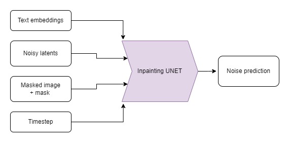
如果我們想保持輸入影像的某些部分不變，但在其他部分生成新的內容呢？這被稱為“inpainting”（影像修復）。雖然這可以用與之前演示相同的模型（透過 StableDiffusionInpaintPipelineLegacy）來完成，但我們可以透過使用一個定製微調的 Stable Diffusion 版本來獲得更好的結果，該版本將蒙版影像和蒙版本身作為額外的條件。蒙版影像應與輸入影像形狀相同，要替換的區域為白色，要保留的區域為黑色。

為了更深入地瞭解 inpainting 過程，讓我們手動實現 StableDiffusionInpaintPipelineLegacy 背後的邏輯。這種方法將闡明 inpainting 在較低層面上的工作原理，並提供對 Stable Diffusion 如何處理輸入的見解。完成此操作後，我們將探索微調的 pipeline 以進行比較。以下是如何手動實現 inpainting pipeline 並將其應用於在“設定”部分載入的示例影像和蒙版的方法：

inpainting from_scratch

DIY Inpainting 迴圈

>>> # Resize mask image
>>> mask_image_latent_size = mask_image.resize((64, 64))
>>> mask_image_latent_size = torch.tensor((np.array(mask_image_latent_size)[..., 0] > 5).astype(np.float32))
>>> plt.imshow(mask_image_latent_size.numpy(), cmap="gray")

>>> mask_image_latent_size = mask_image_latent_size.to(device)
>>> mask_image_latent_size.shape

再次編寫去噪迴圈。

>>> guidance_scale = 8  # @param
>>> num_inference_steps = 30  # @param
>>> prompt = "A small robot, high resolution, sitting on a park bench"
>>> negative_prompt = "zoomed in, blurry, oversaturated, warped"
>>> generator = torch.Generator(device=device).manual_seed(42)

>>> # Encode the prompt
>>> text_embeddings = pipe._encode_prompt(prompt, device, 1, True, negative_prompt)

>>> # Create our random starting point
>>> latents = torch.randn((1, 4, 64, 64), device=device, generator=generator)
>>> latents *= pipe.scheduler.init_noise_sigma

>>> # Prepare the scheduler
>>> pipe.scheduler.set_timesteps(num_inference_steps, device=device)

>>> for i, t in enumerate(pipe.scheduler.timesteps):
...     # Expand the latents if we are doing classifier free guidance
...     latent_model_input = torch.cat([latents] * 2)

...     # Apply any scaling required by the scheduler
...     latent_model_input = pipe.scheduler.scale_model_input(latent_model_input, t)

...     # Predict the noise residual with the UNet
...     with torch.no_grad():
...         noise_pred = pipe.unet(latent_model_input, t, encoder_hidden_states=text_embeddings).sample

...     # Perform guidance
...     noise_pred_uncond, noise_pred_text = noise_pred.chunk(2)
...     noise_pred = noise_pred_uncond + guidance_scale * (noise_pred_text - noise_pred_uncond)

...     # Compute the previous noisy sample x_t -> x_t-1
...     latents = pipe.scheduler.step(noise_pred, t, latents, return_dict=False)[0]

...     # Perform inpainting to fill in the masked areas
...     if i < len(pipe.scheduler.timesteps) - 1:
...         # Add noise to the original image's latent at the previous timestep t-1
...         noise = torch.randn(init_image_latents.shape, generator=generator, device=device, dtype=torch.float32)
...         background = pipe.scheduler.add_noise(
...             init_image_latents, noise, torch.tensor([pipe.scheduler.timesteps[i + 1]])
...         )

...         latents = latents * mask_image_latent_size  # white in the areas
...         background = background * (1 - mask_image_latent_size)  # black in the areas

...         # Combine the generated and original image latents based on the mask
...         latents += background

>>> # Decode latents
>>> latents_norm = latents / pipe.vae.config.scaling_factor

>>> with torch.no_grad():
...     inpainted_image = pipe.vae.decode(latents_norm).sample

>>> inpainted_image = (inpainted_image / 2 + 0.5).clamp(0, 1).squeeze()
>>> inpainted_image = (inpainted_image.permute(1, 2, 0) * 255).to(torch.uint8).cpu().numpy()
>>> inpainted_image = Image.fromarray(inpainted_image)

>>> inpainted_image

Inpainting Pipeline

現在我們已經手動實現了 inpainting 邏輯，讓我們看看如何使用專為 inpainting 任務設計的微調 pipeline。下面是如何載入這樣一個 pipeline 並將其應用於在“設定”部分載入的示例影像和蒙版：

inpainting from_scratch

# Load the inpainting pipeline (requires a suitable inpainting model)
# pipe = StableDiffusionInpaintPipeline.from_pretrained("runwayml/stable-diffusion-inpainting")

# "runwayml/stable-diffusion-inpainting" is no longer available.
# Therefore, we are using the "stabilityai/stable-diffusion-2-inpainting" model instead.
pipe = StableDiffusionInpaintPipeline.from_pretrained("stabilityai/stable-diffusion-2-inpainting")
pipe = pipe.to(device)

>>> # Inpaint with a prompt for what we want the result to look like
>>> prompt = "A small robot, high resolution, sitting on a park bench"
>>> image = pipe(prompt=prompt, image=init_image, mask_image=mask_image).images[0]

>>> # View the result
>>> fig, axs = plt.subplots(1, 3, figsize=(16, 5))
>>> axs[0].imshow(init_image)
>>> axs[0].set_title("Input Image")
>>> axs[1].imshow(mask_image)
>>> axs[1].set_title("Mask")
>>> axs[2].imshow(image)
>>> axs[2].set_title("Result")

當與其他模型結合以自動生成蒙版時，這可能特別強大。例如，這個演示空間使用一個名為 CLIPSeg 的模型，根據文字描述來遮蓋要替換的物件。

補充：管理你的模型快取

探索不同的 pipeline 和模型變體可能會佔滿你的磁碟空間。你可以用以下命令檢視當前下載了哪些模型：

>>> !ls ~/.cache/huggingface/hub/ # List the contents of the cache directory

models--CompVis--stable-diffusion-v1-4
models--ddpm-bedroom-256
models--google--ddpm-bedroom-256
models--google--ddpm-celebahq-256
models--runwayml--stable-diffusion-inpainting
models--stabilityai--stable-diffusion-2-1-base

請檢視關於快取的文件，瞭解如何有效地檢視和管理你的快取。

Depth2Image

depth to image examples 輸入影像、深度影像和生成的示例（圖片來源：StabilityAI）

Img2Img 很棒，但有時我們想建立一個具有原始構圖但顏色或紋理完全不同的新影像。很難找到一個既能保留我們想要的佈局，又不會保留輸入顏色的 Img2Img 強度。

是時候使用另一個微調模型了！這個模型在生成時將深度資訊作為額外的條件。該 pipeline 使用一個深度估計模型來建立深度圖，然後將其輸入到微調的 UNet 中，以（希望）在生成影像時保留初始影像的深度和結構，同時填充全新的內容。

# Load the Depth2Img pipeline (requires a suitable model)
pipe = StableDiffusionDepth2ImgPipeline.from_pretrained("stabilityai/stable-diffusion-2-depth")
pipe = pipe.to(device)

>>> # Inpaint with a prompt for what we want the result to look like
>>> prompt = "An oil painting of a man on a bench"
>>> image = pipe(prompt=prompt, image=init_image).images[0]

>>> # View the result
>>> fig, axs = plt.subplots(1, 2, figsize=(16, 5))
>>> axs[0].imshow(init_image)
>>> axs[0].set_title("Input Image")
>>> axs[1].imshow(image)
>>> axs[1].set_title("Result")

注意輸出與 img2img 示例的比較——這裡有更多的顏色變化，但整體結構仍然忠實於原始影像。在這種情況下，這並不理想，因為為了匹配狗的形狀，這個男人的身體結構變得非常奇怪，但在某些情況下，這非常有用。有關此方法的“殺手級應用”示例，請檢視這條推文，它展示瞭如何使用深度模型為 3D 場景新增紋理！

下一步去哪兒？

希望這讓你體驗到了 Stable Diffusion 的許多功能！一旦你玩膩了這個 notebook 中的示例，可以檢視 DreamBooth 駭客松 notebook，瞭解如何微調你自己的 Stable Diffusion 版本，該版本可用於我們在這裡看到的文生圖或圖生圖 pipeline。

如果你想更深入地瞭解不同元件的工作原理，請檢視 Stable Diffusion 深度剖析 notebook，它會更詳細地介紹並展示一些我們可以做的額外技巧。

請務必與我們和社群分享你的創作！

< > 在 GitHub 上更新

擴散模型課程

簡介

設定